A Comprehensive Survey on Knowledge Distillation

Posted Oct 15, 2026

By Kang TaeYoung

188 min read

출처: TMLR 저자: Amir et al. 연도: 2025 논문: https://openreview.net/forum?id=3cbJzdR78B 코드 / 자료: git-hub

3줄 요약

범위: KD를 포괄적으로 다루며, 기존 Survey들이 간과했던 FM, LLMs, 3D inputs 및 2025 중순까지의 방법론에 대해서 다룸
관점: 기존의 Logit, Feature, Similarity 기반의 분류를 넘어 Adaptive 및 Contrastive Distillation과 같은 최신 알고리즘을 추가하고, 다양한 도메인과 모달리티별로 연구 흐름을 통합적으로 분석
핵심: 최신 연구들을 다각도로 요약·비교하여 향후 연구 방향과 도전 과제를 제시함으로써, Knowledge Distillation 기술의 현재 상태와 미래 발전 가능성을 명확히 정의

A Comprehensive Survey on Knowledge Distillation
Knowledge Distillation(KD, 이후 KD로 통일)연구가 어떤 방향으로 확장되어 왔는가를 파악하는게 핵심 Survey 논문이다.
범위 : KD를 model compression의 관점으로만 바라보지 않는다.
Sources(Knowledge를 무엇으로 바라볼 것인가), Schemes(어떤 Student-Teacher관계로 학습할 것인가), Algorithms(어떻게 전달할 것인가), Modality(어떤 형식의 데이터에 대해 사용할 것인가), Applications(다른 연구분야에 어떤 역할을 하고 적용할것인가)로 설명한다. 이때 이 관점을 독립적인 분야가 아니며, 저자들도 주된 contribution을 주축으로 나누었다고 설명한다. 즉, 각 축이 어떻게 바뀌어왔는지를 중점으로 보면 좋을 듯 하다.
관점의 변화
Knowledge : 초기 KD는 1. 최종 Output, 최종 Prediction이 knowledge였다. 그러나 final prediction만으로는 모델이 도출한 representation을 볼 수 없기 때문에 2. intermediate feature을 전달하는 Feature 을 전달하였다. 이후에는 feature의 값 자체보다 3. sample, class, channel 등의 관계를 옮기는 Similarity를 전달하도록 발전되어 왔다.
Algorithms : 이러한 질문은 근본적으로 “Teacher의 모든 지식을 Student에게 주는것이 맞는가?“라는 질문을 하게 한다. Teacher가 틀릴수도 있고, Teacher와 Student간 Capactiy Gap의 차이가 있을 수 있다. 또한 아키텍쳐가 달라 문제가 발생할 수 있다. 그에 따라 sample, layer, loss, teacher의 기여도를 상황에 따라 조절하는 Adaptive Distillation과 representation space 자체를 구조적으로 맞추는 Contrastive Distillation이 중요해지고 있다.
Teacher : 이렇게 발전되오던 KD는 Teacher가 시대에 따라 변하고 있다.
1 CNN/DNN Teacher → Transformer Teacher → FM / VLM Teacher → LLMs
이 단계에서 부터는 KD의 의미가 단순히 paramter compression을 넘어선다.
VLM(e.g. CLIP) : general-purpose multimodal representation
Segmentation(e.g. SAM) : segmentation capability
SSL(e.g. SimCLR) : label 없이 형성한 representation
Diffusion : iterative generation process
LLMs(e.g. GPT, Qwen) : instruction following이나 reasoning process 정확히는 compression의 의미가 사라진것이 아니라 compression 위에 knowledge/capabiltiy transfer 역할이 확장된 것이다. 특히 LLM계열의 경우에는 cost 문제가 상당하기 때문에 이 두문제가 몹시 중요하다.
각 축의 변화
Sources(무엇을 전달할 것인가?) : 지식이 점점 더 고차원/추상화 되었다.
1 logit → Feature → Similarity
Logit based KD : predict distribution(logit)을 전달하므로 가장 단순하고, 아키텍쳐의 영향이 적다. 그러나 predifined class와 final prediction에 묶여있고, Teacher의 representation을 활용할 수 없다.
Feature based KD : intermediate representation까지 Student에게 전달하여 더 많은 정보를 전달한다. 그러나 아키텍쳐가 다르면서 생기는 문제, 차원 문제 등 어떤 feature을 어떤 feature에 맞춰야하는가와 같은 alignment 문제가 발생한다. 최신의 연구는 이 방향의 해결을 주로 연구하는데(이전은 feature matching → transformation function, cross-layer mixing 등) 이는 Feature based KD가 SOTA의 가능성이 가장 높은 방식이기 때문이다.
Similarity basd KD : 한 단계 더 추상화 시켜서 feature를 맞추기보다 Teacher가 학습한 구조 즉, 관계를 전달하려는 시도가 있다. Instance-level, feature/channel-level, class-level, spatial relation등이 해당한다.
Schemes(Teacher와 Student를 어떻게 구성할 것인가?) : Large2Small의 관점으로만 이해할 수 없다.
1 external large Teacher → peer/ensemble → self
Offline Distillation : 1. Teacher을 먼저 학습 → 2. 학습된 Teacher로 Student학습인 2stage 방식을 사용하며 가장 안정적이고 널리 사용된다. 그러나 Teacher을 준비해야하며 거대한 Teacher을 Studnet학습 내내 실행해야 한다.
Online Distillation : Teacher ↔︎ Student로 pretrained teacher가 반드시 필요하다는 가정을 없앤다. 서로 knowledge를 공유한다.
Self Distillation : Teacher = Student로 변화되었다.
Algorithms(어떻게 전달할 것인가?) : 왜 KD의 확장이 필요할까?
Attention/Graph : 어떤 부분과 관계를 중요시 해야하는가?
Adversarial : distribution alignment나 data-free/robustness 문제까지 KD를 확장
Multi-teacher : 하나의 Teacher가 모든 지식을 가진다는 가정을 버린다.
Cross-modal : Teacher와 Student가 아예 서로 다른 modality를 사용할 수 있도록 확장한다.
Adaptive : Teacher의 지식이 모두 유익하지 않다
Contrastive : 단순 point-wise feature equality보다 representation space의 positive/negative structure를 이용한다.
Modalities(KD를 어디까지 적용시킬 수 있는가?) : 더 좋은 sensor/modality가 training 때만 제공할 수 있는 privileged information을 inference가 싼 modality로 옮기는 도구로서의 KD
1 images → 같은 modality 안에서 model compression → modality 간 knowledge transfer
📌 Applications(KD역할의 확장) : 학습 메커니즘으로 이용
LLMs
1 white box ↔︎ black box
white box(open source) : Logits, hidden state, attention과 같은 기존의 KD사용가능
black box(closed source) : eacher가 만들어 주는 instruction, demonstration, Chain-of-Thought 같은 behavioral output 자체가 knowledge source
Foundation model(FM) : foundation model을 supervision source로 사용하는 것 + model compression
Self Supervised Learning(SSL) : Teacher가 external expert라기보다 Student의 EMA나 다른 view를 처리하는 network가 되면서 KD와 representation learning의 경계쯤 됨. Self Distillation이 주요 방법론
Diffusion : model compression이라기보다 computation/process distillation으로 KD를 이용해 sampling step을 줄이는 방향이 등장
핵심 문제
Knowledge Extraction : Teacher의 logits, features, relation, reasoning중 어느게 실제로 Student에게 유익한지 모름
Capacity gap : Teacher가 강하거나 크기 차이가 너무 크면 오히려 따라갈 수 없음. TA나 Adaptive distillation이 나온 이유
Architecture Difference : Logit은 덜하지만 Feature Distillation 같은 경우 CNN ↔︎ ViT, FM ↔︎ Light model 처럼 아키텍쳐가 다른 경우 alignment가 힘들다
Teacher reliability : Teacher의 잘못된 지식을 학습할 우려
Evaluation comparability : hyperparameter에 매우 민감

A Comprehensive Survey on Knowledge Distillation

제목 + 초록 + 핵심 Figure / Table

2025년도 중반까지의 KD를 정리하는 survey

전통적으로 KD는 아래와 같은 문제제기로 시작한다.

Large DNN / Transformer(FM, LLMs, VLMs, etc.) → High runtime / memory → Deployment difficulty

기존의 survey에 새로운 landscape를 추가한 형식으로 구성되어 있다. Applications에 LLMs, FM, SSl, Diffusion이 추가되었고, Modality에 3D Input이 추가되었다.

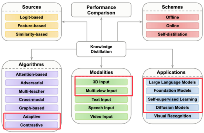
해당 논문의 Fig2

기존의 논문들과의 차이는 아래의 Table과 같다.

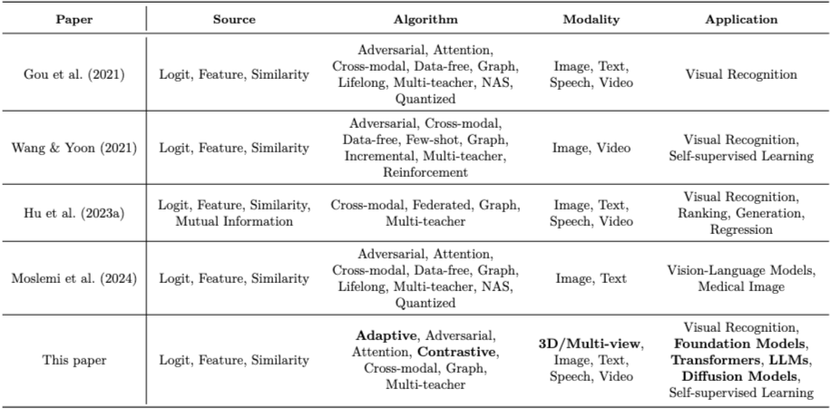
해당 논문의 Table1

이 저자들이 주장하는 이 논문의 핵심은

KD의 최근 적용 범위가 크게 넓어졌기 때문에 기존 KD survey의 틀만으로는 현재 landscape를 설명하기 부족하다

이다.

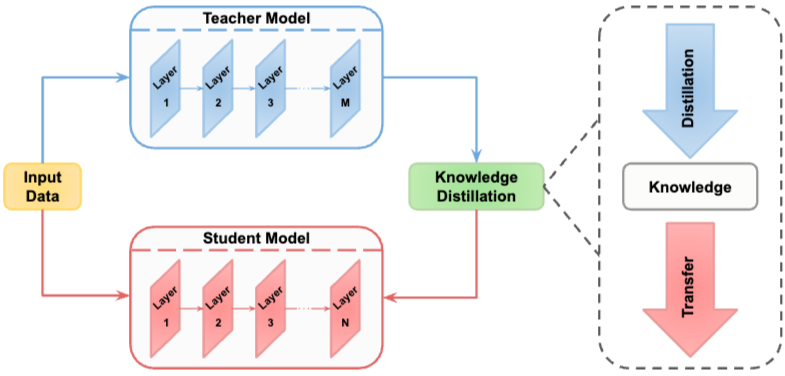
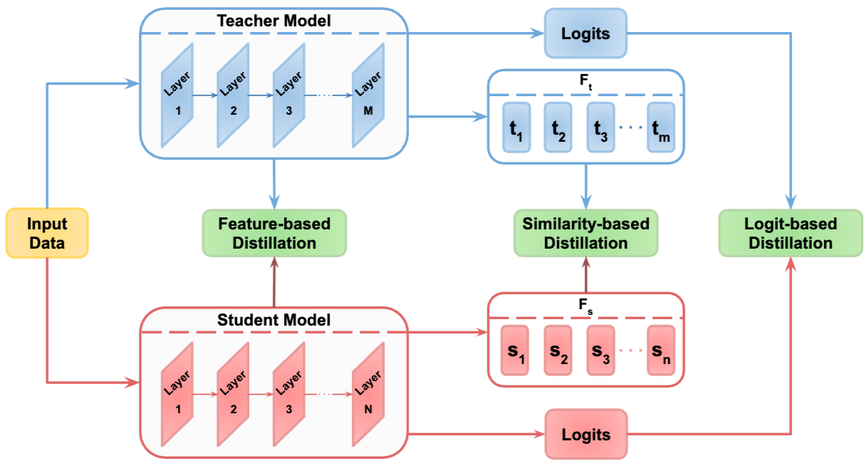
해당 논문의 Fig1

KD의 기본적인 frame work를 잘 설명하는 그림이다. 저자들은 Knowledge 자체를 독립적으로 보고 있다는 점이 이 논문을 관통하는 주요한 내용이다. 즉 3가지의 주체를 가지고 있다. 1. Teacher가 누구인가? 2. 무엇이Knowledge인가? 3.Student에게 어떻게 전달할 것인가?

아래는 논문을 정리하는 주축들이 설명되어있는 그림이다.

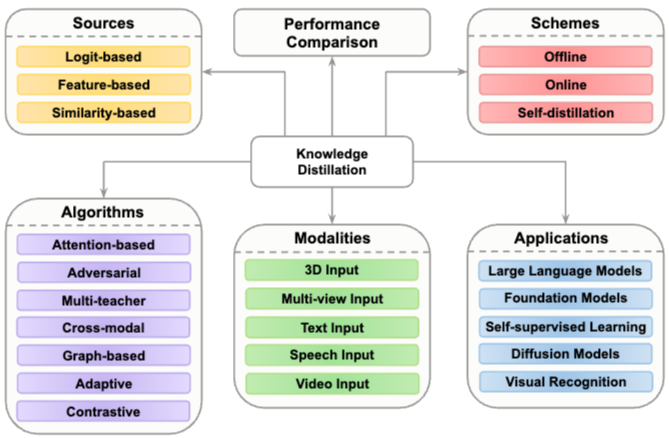
해당 논문의 Fig2

우리는

어떤 KD 방법이 이러한 축에 속하는지 보다 → KD를 설계할때 어떤 dimension들을 결정해야하는가를 집중해야한다.

추가적으로 이렇게 정리한 dimensions는 서로 독립적이지 않으며, 정리 기준은 논문의 주된 기여를 한 축을 기준으로 정리하였다고 한다.

결론 및 Discussion + Future Directions

여전히 KD의 핵심은 Model Compression이나 그 연구분야가 넓어지게 되었다.

최근의 연구들은

Adaptive/Contrastive distillation
3D input
SSL → Self Distillation
Diffusion → sampling step reduction
FM → down stream transfer
LLMs → SLMs 에 대해 이루어지고 있다.

Disscussion

이 Survey에서 분류하는 category들이 서로 베타적인 분류가 아니라, 저자들은 primary contribution을 기준으로 분류한것이라고 한다.

KD의 변화
초기 KD는 model compression에 관점을 두었다면 $T_{pretrained}\ →\ S_{compact}$ 현재는 $\underbrace{\text{무엇을?}}_{\text{Source}} + \underbrace{\text{누구에게서/어떤 관계로?}}_{\text{Scheme}} + \underbrace{\text{어떻게?}}_{\text{Algorithm}}$ 목적에 맞게 여러 설계를 결정해야 한다.

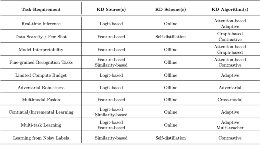
해당 논문의 table 17 : 정답은 아니다

이 표를 통해 저자들은 하나의 universal best KD를 추천하지 않고 task에 맞는 source/scheme/algorithms를 선택해야한다고 주장한다. 저자들이 주장하듯이 SOTA를 위한 접근 방법론인 Feature-based가 Real-time Inference에서 항상 좋은것만은 아니며 Logit based 역시 보편적인 방법론으로 주장한다. 즉 각 사용 사례의 구체적인 목표, 제약 조건 및 맥락 등에 따라 달라진다는 점이다.

다른 연구에서도 그렇지만, KD에서는 특히 정량 비교가 어렵다. 이는 KD의 하이퍼파라미터, Teacher의 checkpoint, dataset, hardware 등 많은 요소가 결과에 영향을 주기 때문이라고 한다. 따라서 저자들이 작성한 Table12 ~ Table 16만을 가지고 단순히 $Method\ A > Method\ B$ 라고 주장하기 어렵고, 어떤 Method가 Best인지는 알 수 없다.

KD는 실용적/윤리적 문제 또한 포함한다.

privacy : KD를 활용해서 model이 training data를 그대로 memorization하거나 sensitive information을 생성할 위험을 줄이려는 연구가 존재한다(data를 직접 노출하지 않고 knowledge를 전달) → 그러나, Data Free Knowledge Distilaltion이라고 해서 privacy가 자동으로 보장되는것은 아니라고 저자들을 주장한다.
fairness, efficiency, sustainability
copyright / intellectual property : Teacher을 이용해 Student를 만드는 행위 자체가 실제 deployment에서는 기술적인 문제뿐만 아니라 법적 문제도 가질 수 있다.

핵심 Challenges

1. Knowledge Extraction

Teacher로부터 무엇을 knowledge로 추출할 것인가

가장 단순하고 효과적인 방버은 logit based distillation이지만, 모든 상황에서 좋지는 않다.

unlabeld setting
중요한 정보가 rich feature, embedding representation LLM에서는 문제가 심해지는데, closed sources model의 경우에는 white box방식의 기존 방식의 KD가 소영이 없고, output만 활용하는 방식으로 밖에 이용할 수 없다.

KD의 인식 변화

How can Student "mimic" Teacher Logits? → What "knowledge" should actually be distilled?

2. Choosing Proper Distillation Scheme

어떤 Teacher Student Scheme을 사용할 것인가

저자들은

FM or Pretrained Large Model → offline
FM or Pretrained Large Model X → online
SSL → self 와 같은 방식들을 설명하고 있다.

또한 Multi Teacher상황에서 trade off로 promising ↔︎ memory, GPU usage가 나타날 수 있다.

그렇긴해도 여전히 offline이 가장 많이 사용된다.

즉, 이러한 상황은 Scheme은 offline → online → self방식대로 발전해온것이 다른 하나를 대체한 것이 아니다. 오히려 다양한 Teacher의 형태가 조건에 따라 나타났다고 보는것이 정확하다.

3. Capacity Gap

Teacher가 더 크고 성능이 좋다고 해서 Student가 항상 더 잘 학습되는것은 아니다.

이는 Teacher와 Student의 size가 지나치게 차이나면 capacity gap이 발생할 수 있기 때문인데, 논문에서는 두 model의 receptive field나 representation capabiltiy가 크게 달라질 수 있기 때문에 Student가 Teacher의 knowledge를 학습하기 어려워질 수 있다고 설명한다.

FM의 경우 capacity gap차이가 훨씬 크기때문에 문제가 심각하다.
Black Box LLMs intermediate layer에 접근할 수 없어 단계적 보정이 어려워 문제가 더 복잡해진다.

이것들을 해결하기 위해 TA나 알고리즘들이 제안되어왔다고 저자들을 설명한다.

4. Architectural Difference

herterogeneous architecture에서의 어떤 layer끼리 같은 semantic information을 가지고 있는지 결정이 어려움

이 문제는 Feature based, Similarity based에서 중요한 문제이다. FM에서는 특히 이 차이가 커질 수 있는데 Teacher와 Student간의 서로 다른 architecture뿐만 아니라 inductive bias 자체가 다를 수 있기 때문이다. 그렇기에 lgoti based는 herterogeneous한 문제에서 상대적으로 대응이 쉬워진다.

black box LLM에 대한 KD에서 CoT distillation이 이 문제에 연결된다고 저자들을 주장한다. 내부 layer을 복제하지 않는 대신, Teacher가 생성한 intermediate reasoning steps를 Student의 supervision으로 사용하지만 reasoing 생성 문제와 Capactiy gap 자체는 여전히 남아 있다.

Future Directions

1. Feature based Distillation

최근 trend와 실험 결과를 근거로 feature based distillaio이 Student 성능 개선에서 중요한 방향이라고 저자들은 평가한다. 동시에 logit과 similarity와 결합할 수 있다.

흥미로운 점은 복잡한 relation을 설계하는 대신, Teacher 또는 Student feature에 비교적 단순한 transformation을 적용한는 것만으로도 강력한 성능을 보인다는 것이다. 일반적으로 $\mathcal{L}_{FD} = D(F_T, F_S)$ 이지만 최근 방향은 사실상 $\mathcal{L}_{FD} = D\left(\Phi_T(F_T), \Phi_S(F_S)\right)$ 으로 $\Phi_T, \Phi_S$를 어떻게 설정할 것인가가 중요한 문제가 된다.

또한 FM에서 얻은 embedding 자체를 Student에게 distill하는 연구도 더욱 중요해지고 있다고 설명한다.

Feature based
Feature based의 변화는
1 더 많은 intermediate feature을 사용 → 서로 다른 representation을 어떻게 연결
로 바뀐거 같다.

2. Adaptive Distillation

Teacher의 의미있는 지식만 정확하게 선택하여 전달하는 문제는 아직 충분히 해결되지 않았다.

Adaptive KD의 목적은 Teacher가 가진 모든 정보를 전달하는것이 아니라 유용한 dark knowledge만 활용하는 것으로 불필요하거나 잘못된 지식을 억제하는 것이다.

Teacher Assistant를 사용하여 capacity gap을 완화
training이 진행될수록 distillation의 influence를 감소
sample importance에 따라 adaptive loss 사용
상황에 따라 Teacher knowledge의 contribution을 조정

Distillation의 발전
Teacher가 더 커지고 Student와의 gap이 커졌기 때문에 모든 knowledge를 동일하게 전달하기 보다 필요한 지식만 전달하는것이 더 필요하다.

3. Distillation from FM

rich knowledge source인 FM, multimodal model들에 대한 KD가 중요하다. 논문에서도 Weakely Supervised Semantic Segmentation을 예를 들며 설명한다. CLIP의 image2text alignment를 이용하면 제한된 visual annotation만을 가지고도 semantic information을 제공할 수 있다.

또한 FM은 open vocabulary task에서도 활용될 수 있다. 즉, 기존 Teacher이 특정 downstream task에서 강하게 학습된 전문가였다면, FM은 보다 넓은 task에 재상요할 수 있는 general representation을 제공한다.

4. Distillation in LLMs

LLM에서의 KD가 다른분야에서보다 더욱 더 필요하다고 한다. LLM의 inference와 deployment cost가 매우 높기 때문에, LLM → SLM에 전달하여 model size를 줄이는것이 중요한 목적이다.

동시에 closed sources인 LLMs가 많아 black box distillation의 중요성이 증가하였다.

CoT Distillation에 저자들이 주목하는데, logit에 Teacher의 reasoing process를 함께 이용하므로서 black box의 intermediation reasoning또한 supervision으로 활용할 수 있도록 한다. 저자들은 이를 활용하면 Studnet의 generaliation을 개선할 수 있음을 강조한다.

LLM 생태계를 만드는 과정에서 KD를 활용하기도 하는데, 큰 LLMs에 pruning이나 quantization을 적용한뒤 KD를 활용하는 방식이며 NVIDIA의 연구와 Qwen3, Gemma3등이 이에 해당한다.

5. Applications of Distillation

독립적인 compression techinque으로만 연구되는 것이 아니라 다른 학습에서도 사용될 수 있다.

adversarial attack / robustness
backdoor attack mitigation
anomaly detection
dataset distillation
quantization과의 결합
low-rank factorization과의 결합

결론적으로

Compression 중심의 KD → 훨씬 다양한 Knowledge / Capabiltiy Transfer까지 포함하는 KD

로 역할이 확장되었다고 보는것이 중요하다.

이는

Teacher가 커지고 범용적이게 됨
전달할 수 있는 지식이 풍부해짐
풍부해짐과는 별도로 capacity와 architeucture gap도 커짐
raw knowledge를 그대로 전달하기 어려워짐
그에 비해 Feautre alignment와 Adaptive selection이 중요해짐
FM/LLM에서 representation과 reasoning까지 그 대상이 확장됨 과 같은 흐름으로 정리할 수 있다.

Teacher의 knowledge를 많이 전달 → Student에게 필요한 knowldege만 전달 가능한 형태로 선택적으로 변환

서론 + Scope

Model compression

FM이나 LLMs들이 등장하면서 training/inference runtime과 memory consumption이 중요한 문제로 떠올랐다. 특히 Edge AI에서의 중요성이 더 크다. Large model의 경우 과매개변수화되어 있는데, 높은 성능을 얻기 위해서 매우 큰 model을 사용하지만 모든 parameter가 동일하게 필수적인 것은 아니다. 이러한 문제를 해결하기 위해 efficient architecture, pruning, quantization, low rank factorization, KD등이 제시되었다.

KD와 Pruning, low rank factorization의 차이 : network의 parameter 또는 structure 자체를 줄이는 pruning과 low rank factorization과 다르게 KD는 더 복잡한 Teacher의 Knowledge를 supervision으로 받아 학습한다. → Model자체를 줄이는것이 아닌, Training supervision을 바꾸는 것

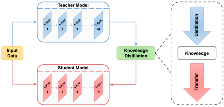
해당논문의 Fig 1

KD는 Teacher가 학습한 knowledge를 student training에 추가적인 supervision으로 사용하는 구조

역사적으로는

Buciluă et al. (2006)의 model compression이 초기 개념을 제시
Hinton (2015)이 Teacher의 output distribution을 soft labels로 사용하여 Student가 이를 mimic하도록 하는 형태를 KD로 널리 확산

Knowledge Transfer

KD의 또다른 목적중 하나는 labeld data 부족으로 인해 target task로 knowledge를 transfer하는 것. Teacher가 Student보다 크다는것이 중요한 것이 아니라 Teacher가 Student에는 없는 useful knowledge를 제공할 수 있다는 점이 중요하다.

Data privacy

Data Free Knowledge Distillation을 사용하므로서 데이터를 직접 저장하거나 사용할 필요 없이 합성 데이터를 생성하여 distillation을 수행할 수 있다.

핵심 challenge

어떤 지식을 전달해야하는가? → Sources
어떤 증류 알고리즘을 사용해야하는가? → Algorithms
어떻게 설계되어야 하는가? → Schemes

기존 KD Survey와 다른점괌 문제점은 아래와 같다.

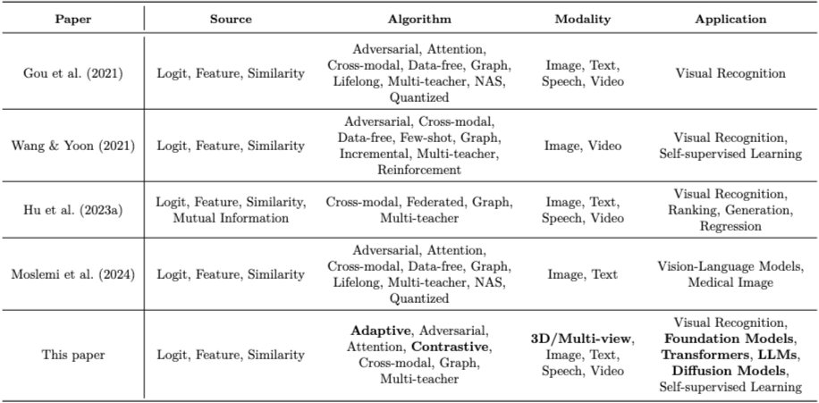
동일 논문의 Table 1

Feature distillation을 충분히 반영하지 않았다.
Adaptive / Contrastive Distillation이 독립적인 연구 방향으로 다뤄지지 않았다.
📌 FM과 LLMs에 대한 KD, 즉 FM과 LLM이 기존의 Teacher보다 훨씬 크고 일반적인 표현이나 multi modal 표현을 가지고 있으며 closed sources일 수 있는데 이를 기존의 전통적인 KD setting에서 다룰 수 없다. 따라서 Applications로 나눠 따로 다뤄야 한다.
📌 3D Input과 같은 최근에 중요해지는 task에 대해 다루지 않았다. → 3D의 경우 정보가 매우 비싼데, cross modal knowledge를 활용한다면 자연스럽게 대쳐할 수 있다. 즉 privileged modality의 knowledge를 다른 modality를 전달하는 도구로의 확장을 보여주는 사례이다.

아래와 같이 survey를 다룬다.

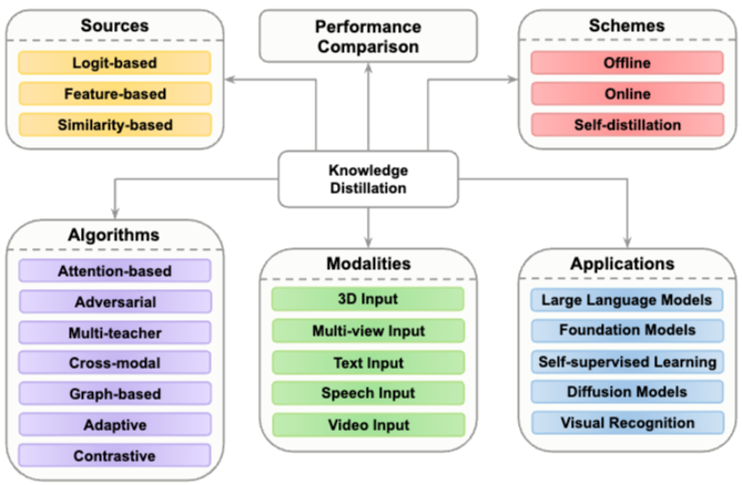
Sources : 무엇을 지식으로 가져오는가
Algorithm : 어떤 방식으로 지식을 전달하는가
Scheme : Teacher와 Student의 관계는 어떻게 되는가
Modaltiy : 전달하고자 하는 지식의 형식은 어떻게 되는가
Applications : KD가 다른 연구에서 어떤 혁할로 사용되는가

Section 2 : Sources

Teacher의 무엇을 knowledge로 전달할 것인가?

Teacher의 어느 위치에서 knowledge를 가져오는가를 기준으로 나눈다.’

[Fig3]

해당 논문의 Fig 3

1. Logit based Distillation

[Table2]

해당 논문의 Table 2

가장 단순한 knowledge source인 Teacher의 마지막 layer output인 logits를 활용한다.

$\mathcal{L}_{ld}(Z_T, Z_S) = \ell_{\text{logit}}(Z_T, Z_S)$ 두 output의 차이를 줄이는 형태이다.

초기 : Soft label

Teacher의 logtis에 temperature $\tau$를 적용하여 soft probabiltiy distribution을 만드는 방식 $p(Z_i, \tau) = \frac{\exp(Z_i / \tau)}{\sum_j \exp(Z_j / \tau)}$ $\mathcal{L}_{ld} = D_{KL}\left(p(Z_T, \tau) \parallel p(Z_S, \tau)\right)$ 그리고 Teacher와 Student distribution 사이의 KL divergence를 최소화 한다. Temperature가 커지면 probability distribution이 부드러워 져서 Teacher가 정답 class 이외의 다른 class에 얼마나 probabiltiy를 주는지 즉 dark knowledge를 포함한다고 Hinton의 표현을 저자들이 인용한다.

최근

Logit Normalization : raw logit scale 차이가 distillation을 방해할 수 있음
- SphericalKD : confidence magnitud 자체가 KD에 반드시 필요한것은 아니라 보고 Teacher-Student gap을 줄임
- NormKD : sample의 logit distribution에 따라 temperature을 조정
- Logit Standardization : logit의 standard deviation 등을 이용해 z score 형태로 normalize
- projector나 temperature 자체를 자체를 분석하는 연구가 많다.
Logit Softening : temperature뿐만 아니라 noise나 별도의 module을 사용하여 Teacher의 prediction을 더 학습하기 쉬운 target으로 만듦
📌 Decoupling : 하나의 KL loss를 의미 있는 components로 분리하는게 최근 많이 연구되고 있다. 이는 Target class와 Target class가 아닌 classes들을 따로 처리해 어떤 부분의 knowledge를 전달하는지 분리하여 제어하는 형식이다.
Revisiting Logit Distillation : 기존 vanila logit KD자체를 다시 분석하여 Teacher Student gap을 줄이는 방법
- TAKD
- VanillaKD
- EffDstl

이러한 LogtiKD의 가장 큰 장점으로 단순하고 직접적이다. 또한 soft output은 규제나 smoothing효과가 있어 overfitting을 줄이는 효과가 있다. 핵심적인 limiation이 있는데

final output중심이기 때문에Teacher 내부에서 prediction이 만들어지는 과정의 intermediate knowledge를 전달하지 못한다.
Teacher와 Student의 architecture/capacity가 다르면 Student가 Teacher의 final prediction만 보고 Teacher의 rich representation을 학습하기 어렵다.

Hinton et al. (2015)

Teacherdml hard prediction이 아니라 temperature을 높인 soft targets를 Student에게 제공한다. 낮은 확률을 받은 incorrect classes 사이의 상대적인 probability도 Teacher가 학습한 generalization structure을 포함한다. Teacher parameter를 복제하는 대신 Teacher behavior을 supervision으로 사용한다.

Logit KD의 발전
Logit KD는 오래된 방식이지만 사라진것이 아니라 문제가 더 정교해졌다.
1 Soft label 사용 → 어떤 logit information을 얼마나 전달할지 제어
특히 normalization과 decoupling을 보면 Teacher output 전체를 무조건 동일하게 따라가는것이 최선이 아니다라는 생각이 여기서부터 나타나는거 같다. 이는 이후 Adaptive Distillation과도 연결된다.

2. Feature based Distillation

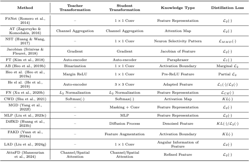
해당 논문의 Table 3

Teacher가 prediction에 도달하기까지 만든 intermediate representation 자체를 knowledge로 전달한다.

DNN의 intermediate layer들은 서로 다른 수준의 representation을 추출한다. 따라서 final prediction만 전달하는것보다 intermediate representation을 함께 제공하면 더 풍부한 knowledge를 전달할 수 있다는 것이 Feature Distillation의 출발점이다. $\mathcal{L}_{fd} = \ell_{\text{feature}}\left(\Phi_T(F_T), \Phi_S(F_S)\right)$ 여기서 중요한 것은 $\Phi_T, \Phi_S$이다. Teacher와 Student의 spatial resolution, channel 수, representation dimension이 같다는 보장이 없기 때문에 feature를 직접 비교하기 전에 transformation / alignment가 필요하다.

초기 : Intermediate Feature 전달

대표 연구는 FitNet으로 Teacher의 intermediate feature를 hint로 사용해 Student가 이를 따라가도록 학습한다. 이후 연구들은 Teacher feature의 어떤 정보를 전달할 것인가를 다양하게 바꾸었다.

AT (Attention Transfer) : feature channel을 aggregation한 attention map
NST : neuron selectivity pattern의 distribution
FT : feature를 factor 형태로 변환
Activation Boundary : neuron의 activation boundary
OFD 계열 : pre-activation feature
CWD : channel-wise probability distribution

즉, $F_T \approx F_S \quad \rightarrow \quad g(F_T) \approx g(F_S)$ 처럼 feature 속 특정 information만 추출해서 전달하는 방향으로 발전했다. Table 3에서 각 method가 Teacher/Student feature에 어떤 transformation을 적용하고 어떤 knowledge와 loss를 사용하는지 비교하고 있다.

Layer Matching : 어느 layer를 어느 layer에 연결할 것인가

Teacher와 Student 모두 여러 layer를 가지므로 초기에는 $F_T^{(i)} \leftrightarrow F_S^{(j)}$처럼 대응 layer를 정해 matching했다. 그러나 이렇게 하면

선택되지 않은 layer의 knowledge는 사용되지 않음
Teacher와 Student의 depth가 다르면 correspondence 자체가 불명확함

그래서 cross-layer feature distillation이 등장한다.

Knowledge Review : Teacher의 feature를 Student의 대응 feature뿐만 아니라 이전 layer들의 information과도 연결
Student feature와 여러 Teacher feature 사이의 연결 weight를 학습하여 one-to-one matching을 일반화

어느 feature를 가져올 것인가? → Teacher와 Student의 representation hierarchy를 어떻게 대응시킬 것인가?

최근

📌 Feature Transformation : 많은 연구의 관심이 feature matching loss 자체보다 transformation function $\Phi$로 이동했다고 저자들은 설명한다.
- Autoencoder : Student feature를 Teacher space로 변환
- MGD : Student feature의 일부 pixel을 masking한 후 convolution으로 reconstruct하여 Teacher feature와 맞춤
- Liu et al. (2023c) : 복잡한 masking 없이 단순 MLP transformation만으로도 충분히 강한 결과를 얻음
- DiffKD : Student feature를 Teacher feature의 noisy version으로 보고 diffusion model로 denoise
- AttnFD : Teacher/Student feature에 channel + spatial attention을 적용하여 discriminative region을 강조한 후 matching
Feature Decomposition : raw feature difference를 magnitude와 angular component로 분해
Feature Augmentation : Student feature를 augmentation하여 Teacher feature와 matching
Frequency Domain : frequency domain에서 feature distillation
N-to-one Matching : 여러 Student feature를 하나의 Teacher feature와 대응
Feature Fusion : Teacher의 모든 feature를 fuse해서 distill

즉, $$\mathcal{L} =

F_T - F_S

\quad \rightarrow \quad \mathcal{L} =

F_T - \Phi(F_S)

$$ 에서 $\Phi$가 무엇이어야 하는가가 중요한 연구 문제가 되었다. 공통적으로 한 layer의 raw tensor를 그대로 복사하는 것에서 벗어나 Teacher representation을 Student에게 맞는 형태로 재구성하는 흐름이다.

Feature KD는 logit보다 더 풍부하고 generalizable한 knowledge를 제공하며, 최근 strong method의 상당수가 feature based라고 저자들은 평가한다. 그러나 그만큼 design choice가 많아지는 제한점이 있는데

어느 layer를 사용할 것인가?
Teacher와 Student의 어느 layer를 대응시킬 것인가?
channel/spatial size가 다르면 어떻게 맞출 것인가?
서로 다른 architecture에서 semantic level이 동일한가?
어떤 transformation을 사용할 것인가?

FM처럼 Teacher와 Student의 architecture와 capacity가 크게 다르면 이 문제는 더 심각해진다. 또한 layer selection, transformation, alignment 설정에 따라 결과가 크게 달라지기 때문에 Feature KD method끼리 공정하게 비교하기도 어렵다고 저자들은 지적한다.

Romero et al. (2014) : FitNets

기존 KD는 Teacher의 final soft output만 사용했고, Student를 더 깊지만 thin한 network로 만들면 optimization 자체가 어려워진다. 이를 해결하기 위해 Teacher의 intermediate representation을 hint로 사용하고, dimension이 다를 수 있으므로 추가 mapping parameter로 Student feature를 Teacher feature에 맞춘다. Final behavior뿐만 아니라 intermediate representation도 knowledge라고 본 전환점이며, 이후 거의 모든 Feature KD의 출발점이다.

Liu et al. (2023) : Channel-wise Transformation

Teacher와 Student feature를 직접 강하게 align하면 Student에게 지나치게 엄격한 constraint가 될 수 있고, 기존 연구는 주로 spatial/pixel-wise alignment에 집중했다. 복잡한 구조 대신 learnable nonlinear channel-wise transformation을 사용해 Teacher-Student representation gap을 맞춘다. Teacher feature를 그대로 복사하는것이 아니라 Student가 학습할 수 있는 representation으로 transform한 뒤 비교한다.

Feature KD에서 바뀐 질문
1 Teacher의 intermediate feature도 따라가게 하면 좋지 않을까? → 서로 다른 Teacher와 Student representation을 어떤 공간에서 비교해야 하는가?
Future Direction에서 본 complex relation design → simple but effective transformation이 여기서 실제로 드러나는거 같다. FM에서 이 방향이 더 중요해지는 이유도 같다. Teacher가 커질수록 knowledge는 풍부해지지만 raw representation은 Student와 더 달라지기 때문이다.

3. Similarity based Distillation

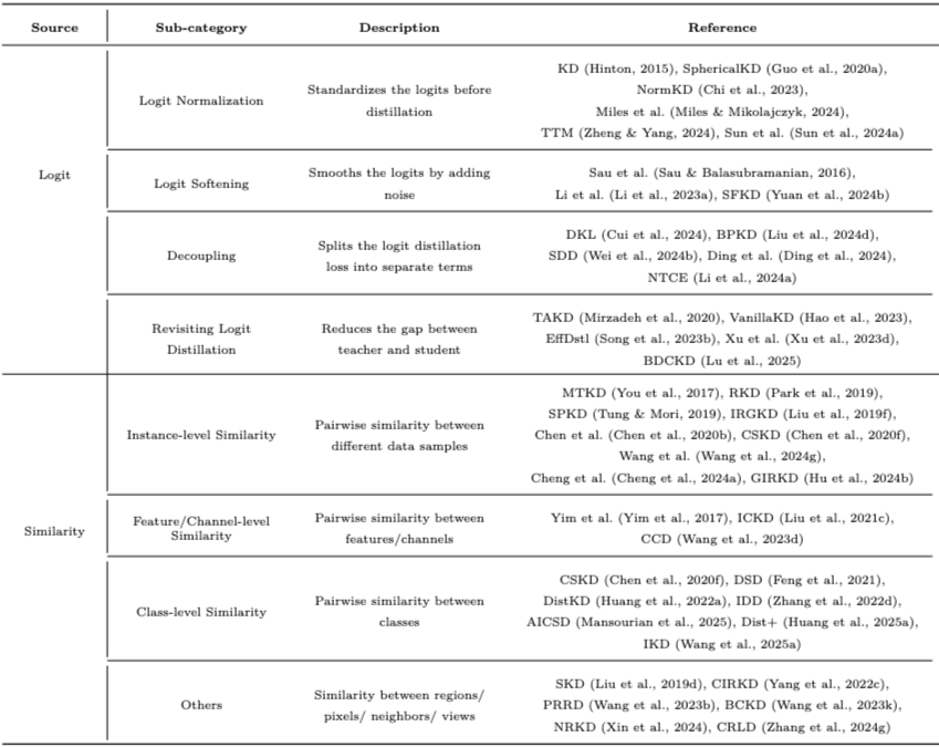
해당 논문의 Table 2

feature의 절대값보다 representation 사이의 관계(structure)를 knowledge로 사용한다.

저자들은 이를 Teacher가 학습한 higher-order structural knowledge를 Student에게 전달하는 것으로 설명한다. $\mathcal{L}_{SD} = \ell_{\text{similarity}}\left(\phi(F_T^i, F_T^j), \phi(F_S^i, F_S^j)\right)$ $F^i, F^j$는 서로 다른 sample이나 layer의 feature/logit, $\phi$는 두 representation 사이의 relation을 계산하고, $\ell_{\text{similarity}}$는 Teacher와 Student relation 사이의 차이를 계산한다. 즉, $F_T^i \approx F_S^i \quad \rightarrow \quad \text{Relation}(F_T^i, F_T^j) \approx \text{Relation}(F_S^i, F_S^j)$ 를 요구하는 형태이다.

초기 : FSP

FSP (Flow of Solution Procedure) 는 Teacher의 서로 다른 두 layer feature 사이의 inner product로 Teacher의 information flow를 나타내고, Student에서도 대응하는 relation을 맞춘다. 이후에는 서로 다른 sample들의 intermediate representation 사이의 relative dissimilarity를 전달하는 연구가 등장한다.

Feature KD : 이 sample의 Teacher feature를 따라가라
Similarity KD : Teacher가 sample A와 B를 서로 어떻게 배치했는지를 따라가라

최근

Table 2에서 relation의 단위에 따라 정리한다.

Instance / Sample level : 여러 sample 사이의 pairwise relation을 전달
- RKD : sample representation 사이의 distance와 angle을 맞춤
- SPKD : batch 내부 sample feature들의 inner product로 pairwise similarity structure를 만들고 유지
- IRGKD : sample feature를 node, relation을 edge로 표현하는 graph 사용
- 📌 CIRKD : batch 내부 relation에 한정되는 문제를 memory bank로 해결하여 global한 sample relation까지 고려
Feature / Channel level : feature channel 사이의 관계를 전달
- ICKD : feature map과 transpose의 dot product로 channel correlation matrix를 만들어 맞춤
- Teacher와 Student의 channel correlation map 차이를 줄이는 연구
Class level : class 사이의 관계를 전달
- DistKD : inter-class / intra-class similarity를 distill
- logit으로 class pairwise similarity를 만들거나, segmentation에서 class별 positional information과 class distance를 전달
- AICSD : class 내부 distribution을 먼저 정의하고, distribution들 사이의 pairwise similarity로 inter-class relation을 distill
Spatial / Region / Pixel level (Others) : dense prediction에서 중요한 spatial structure를 전달
- region-to-region, pixel-to-pixel, pixel-to-region similarity
- neighboring block correlation
- local/global logit similarity

즉 relation의 범위가

Batch local relation → Dataset level / global relation
각 channel 값 자체 → 어떤 channel들이 함께 반응하는가
이 pixel이 class A다 → class A와 B가 Teacher representation에서 어떤 관계를 갖는가

로 확장되었다.

Similarity KD는 Teacher와 Student의 representation space 자체가 같을 필요가 없다는 점에서 architecture가 달라질수록 매력적이다. 하지만 어떤 relation을 정의할 것인가, relation을 계산하기 위한 sample 범위를 어떻게 확보할 것인가(memory bank, graph 등)의 추가 설계 문제가 생긴다.

Park et al. (2019) : RKD

기존 KD는 개별 sample의 Teacher activation을 Student가 그대로 mimic하는 데 집중했다. RKD는 개별 representation이 아니라 여러 sample 사이의 mutual relation을 전달하며, distance-wise와 angle-wise relation을 정의하여 Teacher와 Student의 structural difference를 줄인다. Individual representation이 아니라 representation의 geometry를 전달한다.

Tung & Mori (2019) : SPKD

Teacher에서 비슷하게 활성화되는 두 input은 Student에서도 비슷하게 활성화되도록 pairwise similarity를 보존한다. Student가 Teacher의 representation space 자체를 mimic할 필요 없이 pairwise similarity만 유지하면 된다는 점을 명시한다. $F_T \not\approx F_S \quad \text{여도} \quad \text{Relation}(F_T) \approx \text{Relation}(F_S)$ representation-invariant한 knowledge transfer라는 Similarity KD의 장점을 직관적으로 보여준다.

Similarity KD와 Feature KD의 차이
Feature KD는 Teacher와 Student의 representation을 어떤 방식으로든 정렬해야 하는 문제가 남는다. Similarity KD는 한 단계 추상화해서
1 같은 feature를 만들어라 → 같은 구조를 만들어라

Sources 비교

해당 논문의 Fig 3

Logit : final prediction을 전달 / 단순하고 직접적 / intermediate knowledge를 사용하지 못함
Feature : intermediate representation을 전달 / 더 풍부한 knowledge / layer selection, alignment, transformation 문제
Similarity : sample, channel, class, spatial relation을 전달 / structural, higher-order knowledge / relation 정의와 범위 확보 문제

이것이 세대별로 서로를 대체했다는 뜻은 아니다. Table 12 ~ Table 15의 최신 method들도 Feature + Logit, Similarity + Logit, Feature + Similarity처럼 여러 source를 함께 사용한다. 즉 셋 중 하나를 고르는 문제가 아니라 서로 다른 source의 장점을 결합하는 방향도 활발하다.

Sources의 흐름
1 Output → Representation → Structure / Relation
시간순으로 앞의 방법이 폐기된것이 아니라 knowledge의 abstraction level이 확장된것으로 보는것이 정확하다.
1 2 3 4 5 Logits만 사용 -(Teacher 내부 knowledge를 놓치게 됨)→ Feature까지 전달하는 것으로 확장 Feature 까지 전달 -(Teacher-Student간 representation mismatch 발생)→ alignment/transformation 연구로 확장 Feature 까지 전달 → 절대 feature 대신 relation을 전달하는것으로 확장
FM에서는 Teacher가 더 rich한 embedding을 가지지만 Student와의 차이가 훨씬 커서 이 문제가 더 중요해진다.

Teacher에서 더 많은 정보를 꺼내자 → Student에게 유용하고 전달 가능한 representation을 찾아내자

Section 3 : Schemes

Teacher와 Student를 어떤 관계로 두고 학습할 것인가?

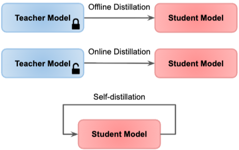
해당 논문의 Fig 4

Section 2가 무엇을 전달할지였다면, Section 3은 Teacher와 Student의 관계를 다룬다.

Offline : Teacher가 이미 학습되어 고정
Online : Teacher와 Student가 동시에 학습
Self : Teacher와 Student가 같은 network/architecture의 서로 다른 상태나 부분

1. Offline Distillation

가장 straightforward하고 가장 널리 사용되는 scheme

두 단계로 학습한다.

Teacher training : 먼저 큰 Teacher를 학습 → $D \xrightarrow{\text{training}} T_{\theta_T}$
Student distillation : Teacher parameter를 frozen한 상태로 Student 학습 → $T_{\theta_T}^{\text{frozen}} \rightarrow S_{\theta_S}$ $\mathcal{L} = \mathcal{L}_{\text{task}} + \lambda \mathcal{L}_{\text{KD}}(T, S)$ Student만 update되며, Hinton식 KD를 포함한 대부분의 전통적인 method가 이 scheme을 사용한다.

저자들은 여전히 가장 많이 쓰이는 이유를 simplicity와 effectiveness로 설명한다. 충분히 학습된 high-capacity Teacher가 있다면 안정적인 knowledge를 그대로 supervision으로 쓸 수 있다. 특히 FM이나 LLM처럼 Teacher를 Student와 함께 재학습하는것 자체가 현실적으로 어려운 경우가 많아 offline이 자연스럽다.

핵심적인 limitation이 있는데

Teacher 실행 비용 : parameter를 update하지 않아도 prediction/feature를 얻기 위해 large Teacher를 memory에 올리고 forward해야 한다. → Teacher frozen ≠ Teacher computation free
Teacher가 고정 : Student 상태에 맞춰 Teacher가 변할 수 없다. Student 성능이 Teacher capability에 제약될 수 있고, Teacher의 bias도 Student에게 전달될 수 있다. 저자들은 offline에서도 Adaptive Distillation으로 Teacher 영향력을 조절하면 도움이 될 수 있다고 연결한다.

LLM의 경우 Teacher가 proprietary model이고 API로만 접근 가능하다면 Teacher training에 참여할 수 없으므로 Teacher를 고정된 external source로 취급할 수밖에 없다. 따라서 offline이 실질적인 선택이 된다.

Offline이 사라지지 않는 이유
FM 시대에는 이미 존재하는 거대한 pretrained Teacher가 많아져서 오히려 offline의 필요성이 분명졌다. 다만 Teacher가 커질수록 trade off도 커진다.
1 Teacher의 강력한 knowledge ↔︎ Teacher forward cost + capacity gap

2. Online Distillation

Teacher와 Student가 같은 training stage에서 동시에 학습한다.

Offline처럼 Teacher pretraining → Student distillation의 두 단계가 아니라 $T_t \leftrightarrow S_t$처럼 training 안에서 knowledge가 만들어지고 동시에 공유된다.

초기 : On-the-fly Teacher

여러 Student/branch의 prediction을 ensemble하여 training 중에 virtual teacher를 만든다. $z_{\text{teacher}} = \text{Aggregate}(z_1, z_2, z_3)$ 이를 다시 각 branch의 supervision으로 사용한다. 즉 완성된 외부 Teacher가 아니라 함께 학습되고 있는 모델들의 knowledge로 Teacher signal을 즉석에서 생성한다.

branch의 의미
여기서 branch는 epoch을 뜻하지 않고, 단순히 Layer 1, 2, 3을 각각 branch라고 하는것도 아니다.
1 Shared or related network → B1 → z1 / B2 → z2 / B3 → z3
한 training system 안의 여러 prediction pathway이며, 여러 독립 network를 쓰는지 하나의 network 안에 여러 branch를 두는지는 method마다 다르다.

최근

이전 prediction 평균 : 이전 prediction들의 평균을 auxiliary supervision으로 사용
Multi depth branch : branch마다 다른 depth를 쓰고, 자신의 prediction뿐만 아니라 여러 branch를 fuse한 prediction을 학습
📌 Contrastive mutual learning : 같은/다른 network의 embedding을 anchor와 비교하며 서로의 representation 학습을 도움
안정성 / generalization : Teacher와 Student의 logit sharpness/variance gap 완화, flatter loss minima
Multi-task / Multi-domain : single-task Teacher나 domain-specific Teacher의 knowledge 활용

즉 Online KD도 단순히 둘을 동시에 학습하는 것에서 끝나지 않고 동시에 변화하는 model들 사이에서 어떻게 안정적이고 유용한 supervision을 만들 것인가로 발전했다.

Guo et al. (2020) : KDCL

전통적인 KD는 large Teacher를 먼저 학습해야 하는 two-stage cost가 있다. KDCL은 모든 network를 Student로 보고 하나의 training stage에서 collaboratively 학습하며, 각 Student prediction을 결합한 soft target으로 서로를 supervision한다. $\text{fixed Teacher} \rightarrow S \quad \Rightarrow \quad S_1 \leftrightarrow S_2 \leftrightarrow \cdots \leftrightarrow S_n$ Teacher를 미리 준비하지 않고 training 과정 자체에서 knowledge source를 만든다.

Online KD의 변화
$\underbrace{K_T = \text{fixed}}_{\text{Offline}} \quad \rightarrow \quad \underbrace{K_T(t) = \text{training과 함께 변화}}_{\text{Online}}$ Teacher를 고정된 model로 보기보다 학습 과정 중 만들어지는 supervision source로 보기 시작한거 같다. 별도의 strong Teacher가 필요 없다는 장점이 있지만, 아직 학습 중인 model들이 서로 가르치기 때문에 supervision 자체가 계속 변하는 안정성 문제가 생긴다.

3. Self Distillation

Online의 특수한 형태로, external Teacher 없이 Teacher와 Student가 같은 network 혹은 같은 architecture에서 유래한다.

다만 $T = S$를 같은 parameter가 같은 순간 자기 자신에게 loss를 건다는 뜻으로 이해하면 너무 좁다. 저자들이 Self Distillation으로 분류하는 방식은 다양하다.

1. 이전 Generation → 새로운 Generation

먼저 $M^{(1)}$을 ground-truth로 학습하고, 같은 architecture지만 다른 random initialization을 가진 $M^{(2)}$에 $M^{(1)}$의 prediction을 distill한다. $M^{(1)} \rightarrow M^{(2)} \rightarrow M^{(3)} \rightarrow \cdots$ Student가 다시 다음 세대의 Teacher가 될 수 있으며, Teacher가 더 큰 architecture가 아니라는 점이 중요하다.

2. 이전 Epoch → 현재 Epoch

과거 prediction을 Teacher로 사용한다. $$p_{\theta_{t-1}}(y

x) \rightarrow p_{\theta_t}(y

x)$$ Kim et al.은 hard target과 previous epoch의 prediction을 linear combination하여 현재 network를 학습한다.

3. Deep Layer → Shallow Layer

하나의 network 내부에서 깊은 부분이 얕은 부분의 Teacher 역할을 한다.

Zhang et al. (2019b) : network를 여러 section으로 나누고 deeper section에서 shallower section으로 knowledge 전달
여러 depth에 shallow classifier를 추가하고 deepest classifier $C_5$의 knowledge를 $C_2, C_3$ 등에 distill

한 iteration 안에서 $C_{\text{deep}} \rightarrow C_{\text{shallow}}$라는 추가 distillation objective가 있는 것으로 보면 된다. 현재 epoch의 Layer 5가 다음 epoch의 Layer 1 weight에 직접 전달되는 구조가 아니며, previous epoch 방식과 deep-to-shallow 방식은 서로 다른 mechanism이다. stop-gradient나 auxiliary head의 구체적인 설계는 method마다 다르므로 원 논문을 확인해야 한다.

최근

Deeper → Shallower
Previous Epoch → Current Epoch
Pruning + Self distillation : model 일부를 반복적으로 pruning하여 Student를 만들고 원래/이전 model의 knowledge를 전달
Graph + Self distillation
📌 Augmentation / View + Contrastive + Self distillation : 같은 sample에 서로 다른 augmentation을 적용해 $x_1, x_2$를 만들고, 같은 semantic을 가져야 하는 representation으로 두어 contrastive learning과 결합 (Xiao et al. (2023b))

Self Distillation ≠ Mean Teacher
different augmentation/view를 쓴다고 Mean Teacher가 되는것이 아니다. Mean/EMA Teacher의 핵심은 $\theta_T \leftarrow m\theta_T + (1-m)\theta_S$ 처럼 Teacher parameter를 Student의 EMA로 update하는 것이다. 이 Survey의 Self Distillation은 previous epoch, deep/shallow, augmentation, pruning 등을 모두 포함하므로 Self Distillation이 곧 EMA Teacher라는 의미는 아니다.

Furlanello et al. (2018) : Born Again Neural Networks

기존 KD는 large Teacher → small Student를 가정했는데, Student가 반드시 작아야 하는지 질문한다. Teacher와 동일한 architecture와 parameterization을 가진 Student를 Teacher output으로 다시 학습시키며, 동일 크기의 Student가 기존 Teacher보다 좋은 결과를 보이는 경우를 보고한다. KD는 compression만을 위한 것이 아니라 training/generalization mechanism일 수 있다.

Self Distillation이 보여주는 변화
Teacher의 정의가 확장되었다.
1 별도의 더 큰 model → 자기 자신의 과거 상태 / 깊은 layer / 다른 view
즉 누가 Teacher인가? 보다 Student보다 더 유용한 supervision을 어디에서 얻을 수 있는가? 로 바뀐거 같다. 또한 Born Again에서 KD ≠ 반드시 model compression이라는 관점이 명확해진다.

Schemes 비교

Offline : pretrained external Teacher / Teacher frozen 후 Student training / 가장 일반적이고 안정적
Online : training 중 형성되는 Teacher 또는 peers / Teacher와 Student 동시 training / 별도 pretrained Teacher 불필요
Self : 같은 architecture/model에서 유래 / 자기 자신의 상태나 부분을 supervision으로 사용 / external large Teacher 불필요

Online과 Self의 차이는

Online : 서로 다른 learner들이 동시에 학습하며 knowledge를 공유 → S1 ↔ S2
Self : knowledge source가 자기 자신에서 유래 → S_past → S_current / S_deep → S_shallow

Schemes의 흐름
Offline → Online → Self를 연도순 대체로 보면 부정확하다. Teacher의 외부 의존성이 점점 완화되었다고 보는것이 더 맞는거 같다.
1 External pretrained Teacher → Training time peers → Self generated supervision
$\begin{aligned} \text{Strong Teacher 준비 비용} &\Rightarrow \text{Online KD} \ \text{External Teacher 의존성} &\Rightarrow \text{Self distillation} \ \text{Label 부족} &\Rightarrow \text{SSL / Self distillation과 결합} \end{aligned}$ 다만 FM / LLM 시대에는 강력한 pretrained Teacher가 이미 있으므로 offline이 다시 자연스러운 선택이다. 결국 Scheme들은 Teacher availability와 training constraint에 따른 서로 다른 해법이다.

Source에서 knowledge의 의미가 Output → Representation → Relation으로 확장되었다면, Scheme에서는 Teacher의 의미가 확장되었다.

고정된 외부 expert → 함께 학습하는 peer → 자기 자신에서 만들어지는 supervision

Section 4 : Algorithms

knowledge를 어떤 mechanism으로 효과적으로 전달할 것인가?

Section 2가 What knowledge?, Section 3이 Teacher-Student 관계였다면, Section 4는 같은 feature/logit을 쓰더라도 How should that knowledge be transferred? 를 다룬다.

Attention based
Adversarial
Multi Teacher
Cross modal
Graph based
📌 Adaptive
📌 Contrastive

Adaptive와 Contrastive는 저자들이 기존 survey에서 독립적으로 다뤄지지 않았던 최근 방향으로 강조하는 부분이다.

1. Attention based Distillation

Teacher의 모든 feature가 동일하게 중요한 것은 아니다.

$F_T \approx F_S$를 요구하면 feature map 전체를 거의 동일하게 취급하게 된다. 반면 attention은 Teacher가 어느 spatial region, 어느 channel을 중요하게 사용하는가를 나타낼 수 있다. 즉 Teacher feature 전체를 복사하는 대신 Teacher가 중요하게 보는 부분을 Student도 중요하게 보도록 만드는 것이 기본 아이디어이다.

What does the Teacher represent? → Where / What does the Teacher focus on?

초기 : Attention Transfer

AT는 convolutional feature를 모두 맞추는 대신 channel을 aggregation하여 attention map을 만든다. $F \in \mathbb{R}^{C \times H \times W} \quad \rightarrow \quad A(F) \in \mathbb{R}^{H \times W}$ 그리고 $A(F_T) \approx A(F_S)$가 되도록 학습한다. 저자들은 이를 Teacher의 neuron selectivity를 반영하는 중요한 region을 Student가 mimic하도록 하는 것으로 설명한다.

최근

Residual Attention : 두 layer feature의 차이/residual에서 attention map을 만들어 representation이 layer 사이에서 어떻게 변하는가까지 전달
Self-Attention aggregation : Teacher/Student feature에 self-attention을 적용하여 context information을 adaptive하게 aggregation
Logit learning을 위한 Attention : logit을 soften하거나 Student가 Teacher output을 쉽게 학습하도록 learning process 자체를 simplify하는 module로 사용
CAM / Grad-CAM : 단순 activation magnitude가 아니라 Teacher가 특정 class를 판단할 때 실제로 사용한 영역을 전달
- channel attention, position/spatial attention, multi level attention, cross-attention으로 확장
📌 Sparse / Cross Attention : Guo et al. (2024b) 은 Student feature를 query, Teacher feature를 key/value로 attention을 계산하고 일부 attention value를 random하게 deactivate하여 sparse attention을 구성한다. 이 attention으로 feature distance의 중요도를 re-weighting하여 negative transfer를 방지한다.
📌 Feature Refinement
- DiffKD : $F_S \approx F_T + \epsilon$로 보고 diffusion으로 denoise하여 중요한 Teacher information을 복원/강조
- AttnFD : Teacher/Student feature 각각에 CBAM(Channel + Spatial Attention) 을 적용한 뒤 refined feature끼리 MSE. segmentation의 small object처럼 discriminative information이 제한된 영역에서 효과적

즉 attention의 역할이

Spatial importance map → KD에서 어떤 information을 강조할지 결정하는 general weighting mechanism

으로 확장되었다.

Zagoruyko & Komodakis (2016) : Attention Transfer

Teacher CNN의 attention을 Student에게 전달할 수 있는지를 문제로 설정한다. full feature tensor를 맞추는 대신 Teacher가 형성한 spatial attention map을 Student가 mimic하게 하여 성능을 개선한다. $F_T, F_S \rightarrow A_T, A_S \rightarrow \mathcal{L}_{\text{AT}}$ feature 자체보다 어디에 주의를 두는지를 전달하는, representation에서 중요한 부분만 추출해 전달하는 대표적인 초기 사례이다.

Attention KD의 위치
Attention KD를 Feature KD와 완전히 별개로 볼 필요는 없는거 같다. $F_T \rightarrow \underbrace{A(F_T)}_{\text{important information}} \rightarrow S$ 처럼 Feature에서 필요한 information을 선택/요약해서 전달하는 algorithm이다. 그래서 AT가 Section 2의 Feature based에도, Section 4의 Attention based에도 등장한다. 분류가 서로 배타적이지 않다는 저자들의 말이 여기서 보인다. 또한 질문이
1 Teacher가 어디를 보는가? → Teacher가 보는 것 중 Student가 실제로 따라가야 할 것은 무엇인가?
로 바뀌면서 Adaptive Distillation과 선택적 knowledge transfer라는 방향에서 연결된다.

2. Adversarial Distillation

adversarial learning을 KD에 사용하는 여러 방법의 묶음

하나의 방법론이 아니라 세 방향으로 나뉘며, 모두 GAN/adversarial learning과 관련있지만 해결하려는 문제가 서로 다르다.

1. Adversarial Data Free KD

Teacher는 있지만 Teacher를 학습한 original data가 없는 경우

privacy, legal constraint, transmission/storage 문제로 $D_{\text{train}}$을 사용할 수 없다면 synthetic input을 생성하여 distillation data 자체를 복원해야 한다. $z \xrightarrow{G} \tilde{x} \xrightarrow{T} \text{Teacher response}, \qquad T(\tilde{x}) \rightarrow S(\tilde{x})$ Generator $G$는 Teacher가 informative한 response를 내는 sample을 만들도록 학습된다. 즉 adversarial learning이 Teacher와 Student를 싸우게 하는 것이 아니라 Student training에 쓸 data를 생성하는 역할을 한다.

그러나 $p_{\text{generated}}(x) \neq p_{\text{original}}(x)$이면 Student가 엉뚱한 영역에서만 Teacher response를 따라가는 문제가 생긴다.

Student의 EMA를 reliable한 learning source로 사용하여 distribution shift 완화
knowledge acquisition과 retention의 균형을 meta-learning으로 다룸
self-adversarial strategy로 robustness 개선
Teacher가 imbalanced dataset으로 학습된 경우를 위한 class-aware generation/distillation

2. Discriminator in the Loop

Teacher와 Student의 output distribution을 더 잘 align하기 위해 discriminator를 사용

discriminator $D$가 Teacher와 Student의 representation을 구별하고, Student는 $D$가 구별하지 못하도록 학습된다. 즉 GAN의 $G \leftrightarrow D$ 구조를 $S \leftrightarrow D$에 적용한 것이다.

Logit level : $Z_T$ vs $Z_S$를 구별
Feature level : $F_T$ vs $F_S$를 구별
더 복잡한 three-player framework

적용 범위도 확장되었다.

GAN Compression : 큰 generator $G_T$를 작은 $G_S$로 압축하면서 generation capability를 보존
📌 Diffusion : Teacher가 여러 denoising step을 수행하지만 Student는 훨씬 적은 step으로 비슷한 output distribution을 만들도록 distill하며, adversarial discriminator로 두 distribution을 align
adversarial score distillation / variational score distillation : score function을 직접 distill

classifier logits / features → generative model output distribution

3. Adversarial Robust KD

Student가 adversarial perturbation에 대해서도 Teacher의 robustness를 물려받게 한다.

일반 KD가 clean input에서 $S(X) \approx T(X)$를 요구한다면, Robust KD는 $X + \delta$를 넣어도 Teacher의 robust prediction과 일치하도록 학습한다. $\min_\theta \mathbb{E}_{(X,y)}\left[\alpha\tau^2 D_{KL}\left(S_\theta^\tau(X+\delta_\theta) \parallel T^\tau(X)\right) + (1-\alpha)\ell(S_\theta(X), y)\right]$ $$\delta_\theta = \arg\max_{

\delta

p < \epsilon} \ell(S\theta(X+\delta), y)$$ Student를 가장 어렵게 만드는 perturbation을 찾고, $S(X+\delta)$가 $T(X)$의 robust target을 따라가도록 한다.

ARD 이후의 발전은

Teacher 신뢰도 : Teacher가 항상 정확/robust하다는 보장이 없으므로 robust soft label을 쓰거나 Teacher를 선택적으로 신뢰
Clean / Adversarial Teacher 분리 : $T_{\text{clean}}, T_{\text{robust}}$ 두 Teacher 사용
Gradient alignment : prediction뿐만 아니라 gradient behavior까지 맞춤
Intermediate adversarial samples : $x \rightarrow x+\delta_1 \rightarrow x+\delta_2 \rightarrow x+\delta_{\max}$를 활용해 natural과 adversarial distribution 사이를 부드럽게 학습
Peer / Dynamic adaptation : Student와 함께 학습하는 peer를 추가하여 상황에 맞는 robust supervision 생성

Teacher robustness를 그대로 복사 → 언제 어떤 Teacher knowledge를 신뢰할지 adaptive하게 결정

세 갈래를 섞지 않는것이 중요하다.

Data Free : original data가 없음 → 어떤 input으로 KD할 것인가?
Discriminator : Teacher-Student distribution mismatch → Teacher와 Student distribution을 어떻게 맞출 것인가?
Robust KD : Student가 adversarial attack에 취약 → 어떤 robustness property까지 전달할 것인가?

Chen et al. (2019) : Data-Free Learning of Student Networks

original training set이 없는 상황에서 GAN으로 Student training data를 만든다. Teacher를 fixed discriminator처럼 사용하고, Generator가 Teacher에서 큰 response를 유도하는 sample을 생성한 뒤 그 data와 Teacher prediction으로 Student를 학습한다. Teacher knowledge를 이용해 distillation용 data까지 생성하여, KD가 original dataset을 반드시 필요로 한다는 가정을 완화한다.

Goldblum et al. (2020) : ARD

KD 과정에서 Teacher의 adversarial robustness가 Student로 얼마나 전달되는가를 연구한다. clean data로 distill해도 robustness의 일부가 전달됨을 관찰하고, 이를 적극적으로 transfer하기 위해 ARD를 제안한다. $\text{Accurate Student} \not\Rightarrow \text{Robust Student}$ KD의 대상이 accuracy뿐만 아니라 robustness 같은 behavioral property까지 확장될 수 있다.

Adversarial KD의 의미
Data Free KD에서는 knowledge extraction 문제와 data generation 문제가 하나로 연결된다. 아무 synthetic data가 아니라 Teacher의 decision knowledge를 드러내는 data를 만들어야 한다. Discriminator 방식은 $ F_T - F_S _2$ 같은 sample-wise matching이 아니라 $p(F_T) \approx p(F_S)$ 같은 distribution-level matching으로 볼 수 있다. 결국 adversarial learning이
1 Data generation / Distribution alignment / Robustness transfer
를 해결하는 도구로 쓰인다. 하나의 기술이 발전했다기보다 GAN framework가 KD의 서로 다른 bottleneck을 해결하는 범용 도구로 흡수된것으로 보는게 맞는거 같다.

3. Multi Teacher Distillation

여러 Teacher의 서로 다른 knowledge를 어떻게 합칠 것인가?

$T_1, T_2, \dots, T_K \rightarrow S$ 서로 다른 Teacher가 서로 다른 knowledge를 가질 수 있으므로 이를 결합하면 Student에게 더 풍부하고 다양한 supervision을 제공해 generalization을 향상시킬 수 있다는 것이 기본 동기이다.

초기 : Prediction Aggregation

여러 Teacher prediction을 하나의 soft target으로 합친다. $p_T = \frac{1}{K}\sum_{k=1}^{K} p_{T_k}$

Hinton (2015) : 여러 Teacher의 logit을 평균하여 softened label 생성
You et al. (2017) : voting strategy
Fukuda et al. (2017) : Teacher pool에서 매번 하나를 random하게 선택
Papernot et al. (2016) : dataset의 서로 다른 subset으로 여러 Teacher를 학습하고 voting

실제 Teacher가 여러 개일 필요도 없다.

Sau & Balasubramanian : 하나의 Teacher logit에 noise를 추가해 $z_T^{(k)} = z_T + \epsilon_k$를 여러 Teacher처럼 사용
TeKAP : pretrained Teacher knowledge를 perturb하여 multiple synthetic teacher knowledge 생성

최근 : Adaptive Knowledge Aggregation

단순 평균은 모든 Teacher가 모든 sample에서 똑같이 좋은 Teacher라는 가정을 가진다. 하지만 Teacher마다 성능, specialization, confidence, architecture, Student와의 capacity gap이 다르다. $p_{\text{teacher}} = \sum_{k=1}^{K} w_k p_{T_k}, \qquad \sum_k w_k = 1$ 핵심은 $w_k = \frac{1}{K}$로 고정하지 않고 Teacher 또는 sample에 맞게 $w_k$를 결정하는 것이다.

Confidence 기반 : Cheng et al. (2024b) 은 Teacher별 KD loss를 분리하고 prediction entropy로 weight 할당 → $w_k = f(H(p_{T_k}))$
Data relation 기반 : Wang & Xu (2024) 는 현재 data가 어떤 Teacher knowledge와 더 관련있는지에 따라 dynamic weighting
Learned aggregation : Zhang et al. (2023a) 은 meta-network로 각 Teacher 사용 정도를 학습, Lin et al. (2024d) 의 adaptive temperature와 diverse aggregation
Expertise 분리 : Teacher마다 다른 종류의 knowledge를 담당
- Chen et al. (2019b) : 한 Teacher는 intricate feature, 다른 Teacher는 general decision feature 전달
- Student 안에 Teacher별 branch를 두어 각 Teacher feature를 학습
- Cao et al. (2023) : 여러 Teacher knowledge를 progressive하게 전달

Hand designed average → Learned aggregation
Prediction aggregation → Feature / Expertise aggregation

📌 Knowledge Amalgamation

Teacher들이 서로 다른 dataset이나 서로 다른 task에서 학습되어 있을 수 있다. 이들의 knowledge를 하나의 Student로 합친다. $T_A(\text{Task A}) + T_B(\text{Task B}) + T_C(\text{Task C}) \rightarrow S_{\text{comprehensive}}$ 저자들은 이미 공개된 pretrained network를 재사용할 수 있다는 점을 중요한 장점으로 든다. Shen et al. 계열에서는 heterogeneous Teacher들이 공유하는 sub-task에서 task-specific knowledge를 먼저 추출한 뒤 합친다.

Multi Teacher의 핵심적인 challenge는

Knowledge Aggregation : $K_{T_1}, K_{T_2}, \dots$를 어떻게 하나의 coherent knowledge로 합칠 것인가
Teacher Contribution : 각 Teacher가 Student에 얼마나 기여해야 하는가 → $w_1, \dots, w_K = ?$
Computational Complexity : 모든 Teacher를 load하고 forward해야 함 → Teacher 수 증가 ⇒ Memory + Compute 증가

즉 knowledge diversity에는 유리하지만 KD의 원래 목적인 efficiency와 training 단계에서 충돌할 수 있다.

Shen et al. (2019) : Amalgamating Knowledge towards Comprehensive Classification

공개된 pretrained model들은 각각 다른 classification problem에 특화되어 있고, 원래 annotation이 없을 수 있다. 서로 다른 task를 담당하는 여러 Teacher의 knowledge를 human annotation 없이 Teacher output만으로 결합하여 모든 class를 처리하는 lightweight Student를 학습한다. $T_1 : \mathcal{T}_1, \quad T_2 : \mathcal{T}_2 \quad \rightarrow \quad S : \mathcal{T}_1 \cup \mathcal{T}_2$ 단순 ensemble이 아니라 서로 다른 expertise를 하나의 model에 통합하는, distributed knowledge reuse로의 확장이다.

Multi Teacher의 변화
1 같은 문제를 잘 푸는 Teacher 여러 개 → 서로 다른 전문가의 knowledge를 한 Student에 통합
Teacher의 역할이 better predictor → specialized knowledge provider로 확장된거 같다. 여기서 중요한 것은 Teacher의 개수보다 knowledge의 diversity이다. 그리고 Teacher가 많아지면 바로
1 그중 지금 이 Student에게 누구의 말을 얼마나 들려줄 것인가?
라는 문제가 생겨서 Adaptive KD와 직접 연결된다. $\text{Knowledge Diversity} \uparrow \quad \leftrightarrow \quad \text{Training Complexity} \uparrow$

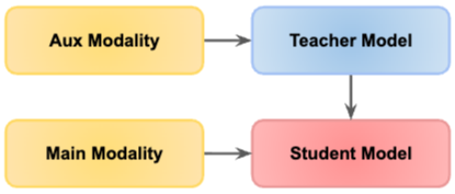
해당 논문의 Fig 5

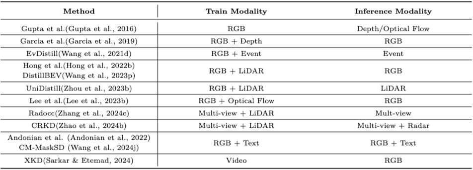
해당 논문의 Table 4

high resource / informative modality의 knowledge를 low resource modality로 전달한다.

한 modality에는 풍부한 annotation이나 강한 representation이 있지만 다른 modality는 그렇지 않을 수 있다. (ex. RGB는 large labeled dataset, Depth는 limited labels) $T_{\text{Modality A}} \rightarrow S_{\text{Modality B}}$ Fig 5가 핵심을 잘 보여주는데, Teacher는 Auxiliary Modality, Student는 deployment에서 쓸 Main Modality를 받는다.

Training : (RGB, Depth) → Depth Teacher의 knowledge → RGB Student
Inference : RGB → Student

즉 비싸거나 사용할 수 없는 modality를 training time privileged information으로 활용할 수 있다.

초기 : Supervision Transfer

Gupta et al. (2016) 은 annotation이 많은 modality에서 annotation이 부족한 paired modality로 supervision을 transfer한다. 두 modality를 parallel stream으로 처리하며 Teacher feature를 Student가 mimic하고, inference에서는 필요한 Student stream만 사용한다.

최근

Modality Gap : $F_{\text{RGB}} \not\sim F_{\text{LiDAR}}$처럼 feature distribution 자체가 다르므로 $

F_T - F_S

$를 단순히 최소화하는 것이 항상 좋은 transfer는 아니다. 이후 연구는 Student output을 Teacher에 더 잘 맞추거나 modality gap을 줄이는 것에 집중했다.

EvDistill : Event ↔ Frame 사이의 bidirectional distillation으로 반드시 단방향일 필요는 없음

📌 2D / 3D : LiDAR는 정확한 geometry/depth를 주지만 sensor cost와 deployment constraint가 있다.
- LiDAR와 RGB 각각에 encoder/decoder를 두고 feature를 align하여 LiDAR의 spatial knowledge를 RGB Student로 distill
- LiDAR 대신 Radar 사용 : spatial information은 적지만 sensor configuration과 비용 측면에서 다른 trade off
- BEV : Camera(perspective image)와 LiDAR(3D point cloud)를 직접 맞추기 어려우므로 $F_{\text{LiDAR}} \rightarrow F_{\text{BEV}}, ; F_{\text{Camera}} \rightarrow F_{\text{BEV}}$처럼 공통 representation space에서 비교
Image ↔ Text
- Andonian et al. (2022) : image와 text feature를 추출하고 aligned instance로 Student supervision
- Wang et al. (2024j) : masking을 사용하고 text feature로 masked image prediction을 guide
Audio ↔ Video
- Sarkar & Etemad (2024) : audio와 video frame을 masking하고 reconstruct하며 두 representation을 align

RGB ↔ Depth → Vision ↔ Language ↔ Audio ↔ 3D / Sensor

Table 4에서는 method 이름보다 Train Modality와 Inference Modality가 어떻게 다른지를 보는것이 중요하다.

Privileged depth : RGB + Depth → RGB
Event transfer : RGB + Event → Event
3D knowledge transfer : RGB + LiDAR → RGB
Optical flow teacher : RGB + Optical Flow → RGB
Camera-Radar : Multi-view + LiDAR → Multi-view + Radar
Image-Text : RGB + Text → RGB + Text
Video transfer : Video → RGB

모든 Cross modal KD가 inference에서 하나의 modality만 쓰는 것은 아니지만, 공통적으로 한 modality에서 얻은 knowledge를 다른 modality의 model learning에 활용한다.

Cross Modality
더 풍부한 모달리티들에서 특정 모달리티만 추출하는 형식으로 진행한다.

RGB에는 ImageNet 같은 대규모 labeled dataset이 있지만 depth나 optical flow에는 없다. 같은 scene의 paired but unlabeled data $(x_{\text{RGB}}, x_{\text{Depth}})$에서 labeled RGB로 학습된 network의 mid-level representation을 supervision으로 사용하여 Depth network를 학습한다. 새 modality에 label을 새로 만드는 대신 다른 modality의 representation을 supervision으로 재사용하는, KD를 compression이 아닌 supervision transfer로 쓴 명확한 초기 사례이다.

Cross modal KD에서 Teacher의 의미
Teacher가 Student보다 단순히 더 큰 model이라서 필요한 것이 아니라 Student가 접근하지 못하는 information을 Teacher가 가지고 있기 때문에 필요하다.
1 capacity superiority → information superiority
서론에서 본 privileged modality의 knowledge를 다른 modality로 전달하는 도구가 바로 이것인거 같다. 또한 Feature KD에서 Teacher Architecture ≠ Student Architecture 때문에 alignment가 중요했다면, 여기서는 Teacher Modality ≠ Student Modality여서 더 심하다. 결국 핵심 질문은 서로 다른 modality를 어느 common representation에서 만날 것인가? 이고, BEV가 대표적인 해답이다.

Multi Teacher는 하나의 Teacher source라는 가정을, Cross modal은 Teacher와 Student가 같은 information source를 가져야 한다는 가정을 완화한다.

Multi Teacher + Cross modal
두 방향 모두 Teacher란 무엇인가? 에 대한 가정을 넓힌것으로 볼 수 있다.
1 하나의 큰 model → 여러 전문가 → 다른 modality의 정보원
현재는 CLIP, SAM, DINO, LLM처럼 서로 다른 strong pretrained model들이 존재하기 때문에
여러 FM의 complementary knowledge를 어떻게 합칠 것인가?
다른 modality의 pretrained knowledge를 target modality로 어떻게 옮길 것인가?
가 중요해진다. 오래된 KD variation이지만 FM 시대에 다시 중요해질 수 밖에 없는 구조적 아이디어인거 같다.

Teacher의 조건 : Student보다 크다 → Student에게 없는 useful knowledge를 제공할 수 있다

5. Graph based Distillation

features 또는 instances 사이의 higher-order relational information을 graph structure로 표현하고 전달한다.

$G = (V, E)$ $V$는 feature 또는 instance, $E$는 그 사이의 dependency/relation이다. $F_T^i \rightarrow F_S^i \quad \Rightarrow \quad G_T(V_T, E_T) \rightarrow G_S(V_S, E_S)$ graph는 local과 global relation을 모두 표현할 수 있어 Teacher의 structured knowledge를 더 풍부하게 전달할 수 있다고 저자들은 설명한다.

graph의 역할은 두 가지이다.

Knowledge structure 표현 : Teacher feature/instance 사이의 relation
Knowledge transfer structure 표현 : 여러 Teacher가 있을 때 각 model을 node로, $T_i \rightarrow T_j$, $T_i \rightarrow S$ 같은 knowledge flow를 edge로 표현

GNN Distillation

GNN 자체를 Teacher/Student로 사용하는 distillation도 중요한 방향이다.

Performance Improvement : KD로 기존 graph model의 성능 향상
Compression : Large GNN → Small GNN, 더 극단적으로는 📌 GNN → MLP로 전달하여 message passing 없이 inference를 단순화 (real-time application)

전달하는 knowledge는 Section 2와 크게 다르지 않지만 connectivity 자체가 추가된다. $\text{Logits} + \text{Feature Representation} + \text{Graph Structure}$

Graph based KD의 위치
Similarity KD가 $\text{Relation}(F_i, F_j)$를 전달했다면, Graph based KD는 이 여러 relation을 하나의 structured graph로 조직한것으로 보면 이해가 쉽다. 새로운 source라기보다 relational knowledge를 더 구조적으로 표현하는 algorithm에 가깝다.
1 representation → relation → structured relation
다만 이번 survey 전체 흐름에서 중심 축이라기보다 Teacher knowledge가 구조까지 포함할 수 있다는 사례 정도로 보는게 적절한거 같다. FM / LLM 흐름과의 직접적인 연결은 Adaptive나 Contrastive보다 약하다.

6. Adaptive Distillation

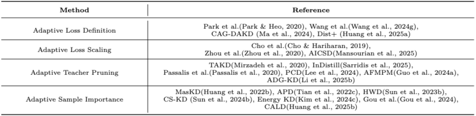
해당 논문의 Table 5

distillation 설정을 고정하지 않고 training 상황에 맞게 dynamically 조절한다.

기존 KD는 $\mathcal{L} = \mathcal{L}_{\text{task}} + \lambda \mathcal{L}_{\text{KD}}$ 에서 $\lambda$, temperature, Teacher contribution, distill할 sample, region/layer 등을 미리 정해두고 training 내내 그대로 사용한다. Adaptive KD는 이를 상황에 맞게 바꾼다. Table 5에서 저자들은 네 범주로 정리한다.

1. Adaptive Loss Definition

Teacher prediction이 항상 정답인 것은 아니다.

Teacher가 틀린 output을 Student가 그대로 mimic하면 Teacher error가 Student에게 전파된다. 따라서 Teacher knowledge가 맞는지에 따라 loss 자체를 다르게 정의한다.

Park & Heo (2020) : Teacher의 probability map이 잘못된 경우 ground-truth로 대체하는 adaptive cross-entropy $\tilde{y} = \begin{cases} p_T, & \text{Teacher가 reliable} \ y, & \text{Teacher가 incorrect} \end{cases}$
Wang et al. (2024g) : Teacher의 잘못된 representation이 간섭하지 않도록 calibrated mask 적용 → $M \odot K_T$
Ma et al. (2024) : 두 Teacher의 positive prediction distribution을 correctness와 cross-entropy magnitude를 고려하여 결합

Teacher를 무조건 신뢰 → Teacher knowledge를 검증한 뒤 사용

2. Adaptive Loss Scaling

Teacher는 training 내내 같은 정도로 필요하지 않다.

Zhou et al. (2020) : training이 진행될수록 distillation loss의 영향을 줄이고, 후반에는 Student 자체가 training을 주도해야 한다고 설명 $\lambda(t_1) > \lambda(t_2) \qquad (t_1 < t_2)$
AICSD : similarity distillation과 vanilla distillation을 결합하면서 weight decay process 사용 $\mathcal{L} = \alpha(t)\mathcal{L}_{\text{similarity}} + \beta(t)\mathcal{L}_{\text{vanilla}}$

Teacher guidance ↑ (초반) → Student autonomy ↑ (후반)

3. Adaptive Teacher Pruning

Stronger Teacher가 항상 Better Teacher는 아니다.

Teacher를 크게 만들면 Teacher의 accuracy는 좋아지지만 Student가 그 knowledge를 이해하기 어려워질 수 있다. $Acc(T_2) > Acc(T_1) \quad \not\Rightarrow \quad KD(T_2 \rightarrow S) > KD(T_1 \rightarrow S)$ Table 5의 이 범주에는 문자 그대로 pruning만 있는 것이 아니라 intermediate model을 넣는 방법도 포함되어 있다.

📌 TAKD : Teacher와 Student 사이에 intermediate-capacity model을 넣음 → $T_{\text{large}} \rightarrow TA_{\text{medium}} \rightarrow S_{\text{small}}$
Passalis et al. : distillation 전에 auxiliary Teacher로 heterogeneous Teacher-Student 사이의 transfer를 도움
Lee et al. (2024) : distillation 전에 Teacher의 channel pruning → $T \rightarrow T_{\text{pruned}} \rightarrow S$
Guo et al. (2024a) : Teacher feature를 pruning하여 Student에게 적합한 knowledge 전달
Sarridis et al. (2025) : filter pruning으로 Teacher channel을 줄이고, layer distillation도 easy layer → hard layer 순서의 curriculum learning

즉 Teacher knowledge를 한번에 그대로 주지 않고 Student가 따라갈 수 있게 difficulty를 조정한다.

4. Adaptive Sample Importance

모든 sample, region, layer가 동일하지 않다.

$w_i \mathcal{L}_{\text{KD}}^{(i)}$ 처럼 단위별로 importance를 다르게 준다.

Sample level
- Tian et al. (2022c) : sample마다 context-specific information 추출
- Sun et al. (2024b) : Student가 혼동하기 쉬운 confusing samples를 찾아 활용
- Kim et al. (2024c) : sample의 energy level에 따라 temperature 조정 → $\tau = \text{const} \rightarrow \tau_i = f(x_i)$
Region / Mask level
- Huang et al. (2022b) : feature distillation에서 mask별 adaptive weight
- Gou et al. (2024) : ground-truth로 중요 region을 mask하고 logit distillation에 집중
Channel level
- Sun et al. (2023b) : Teacher-Student 사이의 channel divergence를 distillation weight로 변환
Layer level
- Kang et al. (2024) : training discrepancy가 큰 layer에 더 큰 weight → $w_l = f\left(D(F_T^{(l)}, F_S^{(l)})\right)$
Class level
- CALD (Huang et al., 2025b) : meta-network로 class-adaptive weight 생성

Sample → Region → Channel → Layer → Class

Table 5의 네 범주를 질문으로 정리하면

Loss Definition : Teacher가 틀린 knowledge를 전달 → 무엇을 믿을 것인가?
Loss Scaling : training 내내 Teacher 영향이 고정 → 언제 / 얼마나 들을 것인가?
Teacher Pruning : Teacher가 Student에 비해 지나치게 복잡 → 누구에게 배울 것인가?
Sample Importance : 모든 sample/region/layer가 동일하지 않음 → 어디에 집중할 것인가?

저자들은 Discussion의 Future Direction에서도 Adaptive Distillation을 다시 선택한다. informative knowledge extraction이 아직 충분히 해결되지 않았고, incorrect/unnecessary knowledge를 피해야 하며, capacity gap을 줄이고, Teacher 영향력을 training에 맞게 바꿔야 하기 때문이다.

Cho & Hariharan (2019) : On the Efficacy of Knowledge Distillation

Teacher accuracy가 Student distillation 성능을 잘 예측하지 못하며, 더 크고 정확한 Teacher가 반드시 더 좋은 Teacher는 아니다라는 것을 실험적으로 분석한다. 원인으로 capacity mismatch를 지적하며, 작은 Student가 지나치게 큰 Teacher를 제대로 mimic하지 못할 수 있음을 보인다. Teacher 자체의 성능 ≠ Teaching effectiveness 라는 관찰이 이후 Adaptive KD 전체의 문제의식을 제공한다.

Mirzadeh et al. (2020) : TAKD

capacity gap이 커질수록 Student 성능이 오히려 떨어질 수 있다는 문제를 다룬다. intermediate-sized Teacher Assistant를 이용한 multi-step distillation을 제안하며, $T \rightarrow TA_1 \rightarrow TA_2 \rightarrow S$처럼 여러 Assistant를 쓰는 형태도 연구한다. knowledge를 한번에 주는 대신 Student가 받아들일 수 있는 난이도로 중간 단계에서 변환한다. → Teacher-centric에서 Student capacity aware teaching으로

Adaptive KD의 의미
기존 KD에는 암묵적으로 Teacher knowledge는 항상 Student에게 도움이 된다는 가정이 있었다. Adaptive KD는 $K_T \neq K_{\text{useful for } S}$일 수 있다고 보고 이 가정을 약화한다. $w = w(x, \text{region}, \text{channel}, \text{layer}, \text{class}, t, \dots)$ 처럼 knowledge transfer의 거의 모든 요소가 adaptive해질 수 있기 때문에, 하나의 algorithm이라기보다 고정된 distillation rule을 버리자는 design principle에 가까운거 같다. 또한 loss weight만 바꾸는게 아니라 Student가 이해하기 쉽도록 Teacher 자체를 바꾸는 것도 포함한다. 즉 더 강한 Teacher가 아니라 더 teachable한 Teacher를 만드는 방향이다.

지금까지의 흐름을 묶으면
$\begin{aligned} \text{Logit} &\rightarrow \text{모든 output 정보가 똑같이 중요한가?} \ \text{Feature} &\rightarrow \text{모든 feature를 그대로 맞춰야 하는가?} \ \text{Attention} &\rightarrow \text{어떤 region/channel이 중요한가?} \ \text{Multi Teacher} &\rightarrow \text{어떤 Teacher를 더 믿어야 하는가?} \ \text{Cross modal} &\rightarrow \text{어떤 representation에서 align해야 하는가?} \ \text{Adaptive} &\rightarrow \text{이 모든 선택을 상황에 맞게 바꾸자} \end{aligned}$ Adaptive는 Logit / Feature / Similarity 어느 source에도, Offline / Online / Multi Teacher 어느 scheme에도 적용될 수 있는 cross-cutting principle이다.

더 많이 전달 → 현재 Student에게 필요한 것을 적절하게 전달

7. Contrastive Distillation

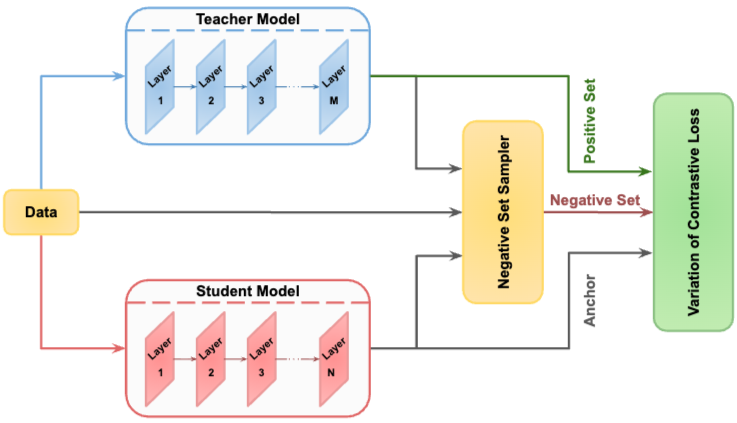
해당 논문의 Fig 6

positive와 negative를 이용해 Student의 representation space 자체를 Teacher와 유사하게 만든다.

Contrastive Learning은 유사한 sample은 가깝게, 서로 다른 sample은 멀어지게 학습하는 방법이며, KD에서는 대부분 feature 기반으로 구성된다.

Anchor : $F_i^S$ (같은 input $x_i$에 대한 Student feature)
Positive : $F_i^T$ (같은 input에 대한 Teacher feature)
Negative : $F_j$ (다른 data point에서 나온 unrelated feature)

$\mathcal{L}_{\text{contrastive}} = -\log \frac{\exp\left(\text{sim}(F_i^S, F_i^T)/\tau\right)}{\sum_{j \in N} \exp\left(\text{sim}(F_i^S, F_j)/\tau\right)}$ $\text{sim}$은 feature similarity, $\tau$는 temperature, $N$은 negative set과 관련된 후보이다. 저자들은 이를 통해 Student feature space를 Teacher feature space와 align할 수 있다고 설명한다. Fig 6에서 negative는 Teacher embedding, Student embedding, input data로부터 구성될 수 있으며, negative를 어디서 가져올 것인가도 algorithm의 일부이다. $\underbrace{\text{Anchor} + \text{Positive} + \text{Negative sampler}}_{\text{구성}} + \underbrace{\text{Contrastive objective}}_{\text{학습}}$

초기 : CRD

Tian et al. (2019)의 CRD 가 선구적인 연구로, 같은 input의 Teacher-Student feature는 positive, 다른 sample의 representation은 negative로 사용해 Student가 Teacher의 representation knowledge를 학습하도록 한다.

최근

WCoRD (Chen et al. (2021b)) : Wasserstein distance의 dual form으로 global knowledge transfer(mutual information 증가), primal form으로 mini-batch 내부 local feature alignment를 동시에 수행
📌 Noisy Negative / Capacity Mismatch : $x_i \neq x_j$라고 반드시 semantic하게 다른 sample은 아니므로 비슷한 sample이 억지로 멀어질 수 있다. 또한 capacity가 크게 다르면 Teacher의 복잡한 embedding geometry를 Student가 따라가기 어렵다. Gao et al. (2021), Fan et al. (2023) 이 이를 고려한 objective를 제안
Dense Prediction (Fan et al. (2023)) : segmentation처럼 수많은 pixel-level representation이 있는 경우 contrastive loss로 feature map을 align → image level instance → dense pixel / region representation
Super Resolution (Liu et al. (2024b)) : Teacher intermediate feature의 statistical information을 contrastive loss로 lightweight Student에 distill
📌 CLIP / VLM (Chen et al. (2024g)) : CLIP 자체가 image와 text를 contrastive하게 align하여 학습했기 때문에 distill할 때도 multimodal feature relationship을 유지하는 contrastive objective가 자연스럽다. image feature alignment와 educational attention을 사용
NLP (DistilCSE) : large contrastive sentence embedding model을 작은 model로 압축
Medical Imaging (CRCKD, Xing et al. (2021)) : class-guided contrastive distillation과 categorical relation preserving을 결합하여 intra-class similarity와 inter-class divergence를 높임. class centroid와 relational graph를 사용하며 imbalanced dataset에서도 효과적
Weakly Supervised Visual Grounding (Wang et al. (2021e)) : detector의 pseudo-label을 이용해 region ↔ phrase matching에 contrastive loss를 적용하여 inference 시 detector가 필요없도록 함
Relation Contrast (CRCD, Zhu et al. (2021b)) : raw representation이 아니라 inter-sample relation distribution 자체를 contrastively align $R_T(i,j) = \text{Relation}(F_i^T, F_j^T), \quad R_S(i,j) = \text{Relation}(F_i^S, F_j^S)$
CRD (Zhu et al., 2025) : sample-wise similarity를 보존하는 intra-sample alignment와 structural semantic을 포착하는 inter-sample contrast로 class-wise semantic alignment 강화

CRD → Global + Local (WCoRD) → Dense / SR / Medical / NLP → CLIP multimodal → Relation / Class semantic structure

저자들은 Contrastive KD의 강점을 feature alignment, relational knowledge preservation, local/global information integration에서 찾는다. multi-modal alignment, dense feature mapping, model compression뿐만 아니라 imbalanced dataset, noisy label, computational constraint에도 적용 가능하며, 특정 architecture에 묶이지 않고 representation relation을 정의할 수 있는 다양한 task에 적용 가능한 flexibility가 장점이다.

Similarity KD와 헷갈리기 쉬운데 둘은 서로 다른 축이다.

Similarity based : Source → Teacher의 무엇을 가져오는가? → relation / similarity
Contrastive : Algorithm → 어떻게 학습시키는가? → positive / negative contrast

따라서 Contrastive KD는 raw feature도, relation도 사용할 수 있으며 저자들은 대부분이 feature based contrastive learning이라고 설명한다.

Tian et al. (2019) : CRD

KL divergence 기반 KD는 probabilistic output은 전달하지만 Teacher representation에 존재하는 structural knowledge를 충분히 전달하지 못한다. Teacher와 Student representation 사이의 mutual information을 키우는 문제를 contrastive objective로 구성하여 $(F_i^S, F_i^T)$는 positive, $(F_i^S, F_j^T), ; i \neq j$는 negative로 둔다. compression뿐만 아니라 ensemble distillation, cross-modal transfer에서도 평가한다. Output imitation → Representation discrimination transfer로의 전환이다.

Chen et al. (2021) : WCoRD

KL 기반 KD가 structural knowledge를 충분히 포착하지 못하고, Teacher와 Student가 다른 classification task를 다루면 feature generalization이 제한된다는 문제에서 출발한다. dual formulation은 mutual information lower bound를 높이는 contrastive objective와, primal formulation은 mini-batch 내 feature distribution alignment와 연결된다. Global contrastive transfer + Local distribution matching을 함께 전달한다.

Chen et al. (2024) : ComKD-CLIP

큰 CLIP은 strong multimodal representation을 가지지만 resource-limited 환경에 배포하기 어렵고, 작은 CLIP은 성능이 부족하다. IFAlign은 Student image feature를 Teacher image feature에 맞추고, EduAttention은 Teacher text feature와 Student image feature 사이의 cross-relationship으로 Teacher가 image와 text를 결합하는 knowledge까지 학습하게 한다. 전달 대상이 visual representation 하나가 아니라 Image-Text 관계 자체가 되는 FM 시대의 변화를 보여준다. (Section 6 FM에서 다시 확인)

Gao et al. (2021) : DistilCSE

large contrastive sentence embedding model은 online serving 비용이 크다. 대량의 unlabeled data로 먼저 distill한 뒤 limited labeled data로 contrastive fine-tuning하며, CKD에 InfoNCE objective를 사용해 Teacher training → KD → Student fine-tuning 사이의 objective consistency를 높인다. Teacher가 contrastive하게 학습되었다면 transfer 과정도 contrastive objective와 맞춘다.

Contrastive KD의 변화
1 Teacher feature의 값 자체를 복사 → Teacher가 만든 representation space의 구조와 구별 능력을 전달
$F_T \approx F_S \quad \rightarrow \quad \text{Geometry / Relation}(F_T) \approx \text{Geometry / Relation}(F_S)$ 그래서 exact tensor matching에 덜 의존하고, representation space 자체가 중요한 FM이나 multimodal embedding과 특히 잘 연결되는거 같다. CLIP이 image ↔ text의 상대적인 embedding geometry를 contrastive로 학습했는데 $F_T \approx F_S$만 강제하면 cross-modal relational structure의 일부를 놓칠 수 있다. DistilCSE처럼 knowledge의 값뿐만 아니라 knowledge가 형성된 objective까지 고려해야 한다. 또한 여기서도 모든 negative를 동일하게 취급해도 되는가? 라는 문제가 나오는데, Adaptive KD에서 본 모든 Teacher knowledge가 유용하지 않다와 같은 문제가 반복되는 것이다.

Adaptive와 Contrastive가 최근 중요해진 이유
둘은 FM 시대의 두 문제와 대응하는거 같다.
Teacher가 너무 강하고 거대해짐 → 모든 knowledge를 그대로 전달할 수 없음 → Adaptive = Selective Transfer
Teacher가 훨씬 rich한 embedding space를 가짐 → output보다 representation structure를 보존해야 함 → Contrastive = Structural Representation Transfer

Algorithms 정리

\[\begin{aligned} \text{Attention} &: \text{무엇을 강조할까?} \\ \text{Adversarial} &: \text{data / distribution / robustness 문제를 어떻게 맞출까?} \\ \text{Multi Teacher} &: \text{여러 Teacher knowledge를 어떻게 합칠까?} \\ \text{Cross modal} &: \text{다른 modality의 knowledge를 어떻게 연결할까?} \\ \text{Graph} &: \text{관계 구조를 어떻게 전달할까?} \\ \text{Adaptive} &: \text{무엇을 언제 얼마나 전달할까?} \\ \text{Contrastive} &: \text{representation structure를 어떻게 보존할까?} \end{aligned}\]

Feature를 source로 정했다고 끝나는 것이 아니라, $F_T$를 그대로 matching할 수도, attention으로 중요한 부분만 고를 수도, discriminator로 distribution을 align할 수도, contrastive하게 구조를 전달할 수도 있다. 즉 최근 KD의 발전은 knowledge source와 transfer mechanism이 동시에 세분화되는 과정이다.

Teacher output을 단순히 mimic → knowledge의 중요도, 구조, source, modality, training state를 고려해 가공해서 전달

Section 5 : Modalities

KD가 어떤 종류의 data까지 확장되었는가?

앞의 Source / Scheme / Algorithm이 KD 자체를 어떻게 설계할 것인가였다면, Section 5는 KD가 image 이외의 어떤 data로 확장되었는지를 다룬다. 서론에서 본 것처럼 3D Input과 Multi-view Input은 저자들이 기존 survey와의 차별점으로 강조한 부분이다.

1. 3D Input

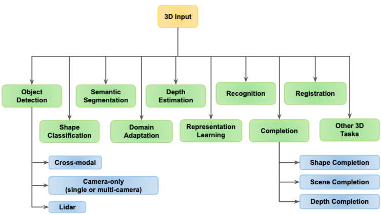
해당 논문의 Fig 7

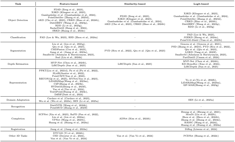
해당 논문의 Table 6

3D에서 KD는 특정 task의 기법이 아니라 3D perception 전반에서 쓰이는 learning framework이다.

Fig 7은 3D KD를 algorithm이 아니라 3D task의 종류에 따라 정리한다.

3D Object Detection (LiDAR / Camera-only / Cross-modal)
Shape Classification
Semantic Segmentation
Domain Adaptation
Depth Estimation
Representation Learning
Recognition
Completion (Shape / Scene / Depth)
Registration

3D data에는 image와 다른 고유한 문제가 있다. $\text{Sparsity} + \text{Occlusion} + \text{Varying Density}$ LiDAR point cloud는 공간을 dense하게 관측하지 않고, object가 가려질 수 있으며, sensor configuration과 거리에 따라 density가 달라진다. 그래서 일반적인 2D feature KD를 그대로 적용하기 어렵다. 또한 point-wise label이나 3D bounding box 같은 3D annotation은 비용이 매우 높다.

3D Object Detection

3D에서 가장 자세히 다뤄지는 영역으로 세 방향으로 정리한다.

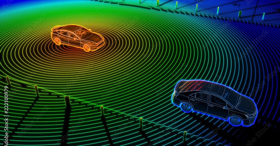
https://www.yellowscan.com/knowledge/lidar-for-cars-understanding-the-core-technology/

LiDAR : sparsity와 occlusion 문제를 강한 Teacher의 richer geometric representation으로 보완
- X-Ray Distillation : 여러 LiDAR scan을 aggregation한 object-complete frame을 Teacher input으로 쓰고, Student는 실제 관측되는 sparse frame에서 학습
- LiDAR Distillation : high-beam LiDAR Teacher → low-beam LiDAR Student
Camera-only : camera만으로는 직접적인 depth information이 부족하다.
- FD3D : perspective와 BEV space에서 object-specific knowledge를 selective masked generative distillation과 focal distillation으로 전달
- X3KD : Cross-task + Cross-modal + Cross-stage distillation을 함께 사용
📌 Cross-modal : LiDAR는 정확한 depth와 geometry를 주지만 sensor cost와 deployment constraint가 크다. 따라서 LiDAR 또는 LiDAR+Camera Teacher의 knowledge를 Camera(+Radar) Student로 전달한다.
- CRKD : LiDAR-camera Teacher → camera-radar Student
- DistillBEV : LiDAR Teacher → multi-camera BEV Student
- CMKD : LiDAR Teacher → monocular Student
- UniDistill : LiDAR ↔ Camera 등 여러 modality pair 지원

Cross-modal에서는 많은 method가 BEV를 공통 representation으로 사용한다. $F_{\text{LiDAR}} \rightarrow F_{\text{BEV}}, \qquad F_{\text{Camera}} \rightarrow F_{\text{BEV}}$ modality가 달라도 같은 geometric coordinate로 projection한 뒤 knowledge를 전달한다.

3D Semantic Segmentation

point cloud의 sparsity, randomness, varying density 때문에 일반적인 distillation이 어렵다.

PVD 계열 : fine-grained point knowledge와 coarse structural voxel knowledge를 함께 활용 → Point level detail + Voxel level structure
Qiu et al. : multi-scan의 richer information을 single-scan Student에 전달하며 feature / logit / instance similarity를 함께 사용

또한 point-wise annotation이 매우 비싸기 때문에 self-distillation이나 외부 pretrained model을 활용한다.

📌 Seal : off-the-shelf Vision Foundation Model → point cloud segmentation
📌 PartDistill : Vision-Language Model → 3D segmentation

2D Foundation Model → 3D Model

📌 3D Representation Learning

저자들은 두 가지 현실적인 문제를 강조한다.

large high-quality 3D annotated dataset 수집이 비쌈
large-scale 3D dataset이 부족해서 3D model을 대규모로 pretrain하는 것 자체가 어려움

반면 2D에는 이미 large-scale dataset, pretrained model, FM이 존재한다. 따라서 PPKT, SLidR, PointCMT, RECON, HVDistill, Text4Point, Diff3F 등이 2D model의 knowledge를 3D point cloud representation으로 distill한다. $\text{2D Semantic Representation} \rightarrow \text{3D Representation}$

나머지 3D Task

Shape Classification : feature / logit / self-distillation으로 point cloud classifier의 representation과 robustness 개선
Domain Adaptation : label이 있는 source domain → label이 없는 target domain에서 self-distillation이나 cross-modal feature fusion 사용
Depth Estimation : RGB, radar, point cloud의 geometric information을 distill하여 lightweight depth estimator 학습
Recognition : Visual Place Recognition에서 image ↔ LiDAR cross-modal KD
Completion : 불완전한 point cloud / scene / depth를 복원할 때 Teacher의 learned prior를 전달하여 missing geometry 예측
Registration : large model의 point cloud matching knowledge를 compact model로 전달하거나 self-distillation
기타 : generation, stylization, sampling

Table 6에서 각 3D task의 method를 다시 Feature / Similarity / Logit으로 정리한다. 즉 3D라고 새로운 source taxonomy가 생기는 것이 아니라 Section 2의 분류가 그대로 적용되고, 3D geometry와 modality 차이 때문에 어떤 feature, relation, spatial representation을 distill할지가 달라질 뿐이다.

task 이름은 많지만 반복되는 목적은 몇 가지이다.

Sparse / incomplete 3D observation 보완
3D annotation 부족 보완
stronger modality의 geometry / semantics 전달
3D model inference cost 감소

Wang et al. (2023) : DistillBEV

multi-camera BEV detector는 production cost가 낮지만 depth와 geometry를 직접 측정하지 못해 LiDAR detector와 성능 차이가 있다. LiDAR Teacher와 camera Student를 모두 BEV representation에서 만나게 하여 modality gap을 줄이고, foreground/background decomposition, object size에 따른 adaptive scaling, spatial attention, multi-scale feature distillation, temporal fusion으로 중요한 geometric region을 선택적으로 전달한다. LiDAR Teacher는 training에만 사용되므로 inference에서 추가 LiDAR computation이 없다. Cross-modal + Feature + Attention + Adaptive weighting이 한 method에 결합된, 하나의 category로 설명하기 어려운 최근 KD의 전형이다.

Sautier et al. (2022) : SLidR

autonomous driving에서 point cloud annotation은 매우 비싸다. 차량에는 camera와 LiDAR가 synchronized/calibrated되어 함께 장착되어 있다는 점을 이용해, self-supervised pretraining된 image representation을 LiDAR로 distill한다. 단순 pixel-to-point가 아니라 superpixel 단위의 visually coherent region에서 2D feature와 3D point feature를 contrastive하게 align하며, image와 point cloud 모두 semantic annotation이 필요 없다. Self-supervised + Cross-modal + Contrastive + 2D → 3D로, KD가 compression이 아니라 annotation이 부족한 modality의 pretraining mechanism으로 쓰인 사례이다.

3D에서 KD가 자연스러운 이유
3D에는 두 문제가 동시에 있다.
1 좋은 3D supervision은 비쌈 + 강력한 2D model과 data는 이미 많음
그래서 2D / LiDAR / Multi-modal Teacher → 3D Student가 자연스럽고, 3D에서 KD는 large 3D model compression보다 다른 modality에 이미 있는 knowledge를 3D learning에 활용하는 역할이 더 중요한거 같다. 또한 LiDAR Distillation이나 X-Ray Distillation을 보면 Teacher와 Student의 차이는 model size가 아니라 Teacher가 더 좋은 observation을 본다는 것이다. Camera Student도 parameter가 작은게 문제가 아니라 input 자체에 명시적인 3D geometry가 없다는게 문제이다.
1 Teacher의 우월성 : Model Capacity → Data / Sensor Quality
DistillBEV도 결국 inference 때 쓸 수 없는 richer sensor의 geometry를 training supervision으로만 사용한 것이다.

2. Multi-view Input

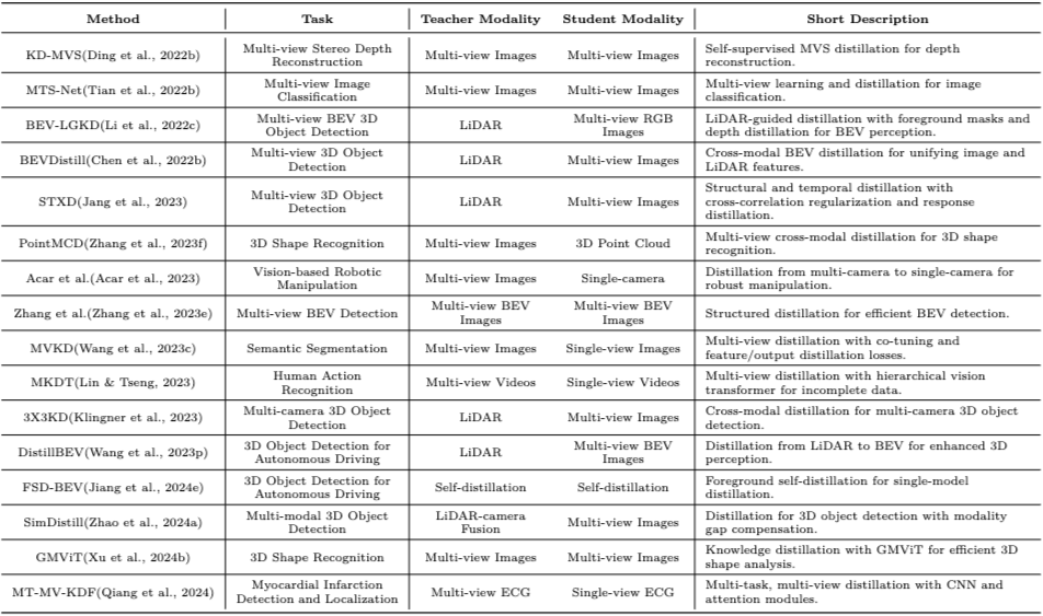
해당 논문의 Table 7

여러 viewpoint가 주는 complementary information을 효율적인 Student에게 전달한다.

$x^{(1)}, x^{(2)}, \dots, x^{(V)}$를 함께 쓰면 single view로는 얻기 어려운 정보를 활용해 더 정확하고 robust한 representation을 만들 수 있다. 그러나 두 가지 문제가 있다.

여러 view를 모두 처리하면 computational cost가 증가
서로 다른 view / modality의 knowledge를 어떻게 하나의 Student에 전달할지 결정해야 함

3D Object Detection

multi-camera image로 BEV representation을 만들 수 있지만 camera만으로는 depth/geometry 추론이 어렵다. 그래서 대부분 $T_{\text{LiDAR}} \rightarrow S_{\text{Multi-view RGB}}$ 형태로 LiDAR의 accurate geometry를 전달하고 inference에서는 camera만 사용한다. (BEV-LGKD, BEVDistill, STXD, X3KD, DistillBEV, SimDistill 등)

BEV-LGKD : LiDAR point를 BEV에 projection하여 foreground mask를 만들어 RGB BEV model을 guide하고, depth distillation으로 depth estimation 능력 강화
BEVDistill : image와 LiDAR를 BEV common space에서 통합하고 heterogeneous representation 사이에서 adaptive하게 knowledge 전달
📌 STXD : spatial feature뿐만 아니라 multi-frame $F_t, F_{t-1}, \dots$ 사이의 temporal relation을 similarity map으로 전달 → spatial → spatio-temporal
FSD-BEV : external Teacher나 복잡한 cross-modal Teacher 없이 self-distillation 사용

즉 Multi-view ≠ 반드시 external multi-modal Teacher이며, Scheme과 Modality 축이 다시 결합되는 사례이다.

3D Shape Recognition

3D object는 3D Point Cloud 또는 Multiple 2D Views로 표현할 수 있다. multi-view image representation이 강력한 visual information을 제공하므로 이를 point cloud encoder에 distill하며, 대표 method가 PointMCD이다.

Other Tasks : Multi-view → Single-view

training에서는 여러 view를 쓰고 inference에서는 하나만 쓰는 패턴이 중요하다.

Acar et al. : robotic manipulation에서 multi-camera policy → single-camera policy
semantic segmentation, human action recognition, medical ECG, multi-view classification 등에서도 등장

Table 7은 method를 Task, Teacher Modality, Student Modality로 정리하는데, method 이름보다 Teacher가 무엇을 더 볼 수 있고 Student는 실제로 무엇만 쓸 수 있는가를 보는것이 중요하다.

LiDAR → Multi-view RGB : geometry transfer
Multi-view Image → Point Cloud : 2D visual → 3D geometric knowledge
Multi-view Camera → Single Camera : inference sensor 감소
Multi-view Video → Single-view Video : view 부족 보완
Multi-view ECG → Single-view ECG : rich observation → efficient inference

Zhang et al. (2022) : PointMCD

point cloud는 irregular geometric signal이라 discriminative feature 추출이 어렵고, 여러 benchmark에서 multi-view image 기반 representation이 더 강한 경우가 있다. $T_{\text{Multi-view 2D}} \rightarrow S_{\text{3D Point Cloud}}$로 전달하는데, 2D feature와 3D feature는 형태가 전혀 다르므로 visibility-aware feature projection으로 3D point representation을 각 view에 대응하는 descriptor로 aggregation한 뒤 view별로 pairwise align한다. 2D와 3D tensor를 억지로 맞추는 대신 서로 비교 가능한 view-specific representation으로 변환한 뒤 distill한다.

Multi-view KD의 핵심
Multi-view는 Information ↑이지만 동시에 Sensor / Compute Cost ↑이다. KD를 이용하면
1 Training : multi-view의 정보량 사용 → Inference : single / fewer view의 비용만 사용
할 수 있고, 이는 Cross-modal KD에서 본 rich training information → cheap inference와 같은 원리인거 같다. Perspective views → BEV가 자주 쓰이는 이유도 서로 다른 sensor/view의 knowledge를 같은 coordinate에서 align하기 좋기 때문이다. PointMCD에서도 Feature KD의 문제가 반복된다. rich Teacher feature가 있어도 Student representation과 직접 비교할 수 없으면 쓸 수 없다. 결국 최근 KD의 핵심은 Knowledge Extraction + Knowledge Alignment로 모이고 있다.

3D와 Multi-view에서 반복되는 패턴은

Strong sensor → Weak / Cheap sensor : LiDAR → Camera / Radar
Dense / Rich observation → Sparse observation : High-beam / Aggregated LiDAR → Sparse LiDAR
Multiple views → Fewer views : Multi-view → Single-view
Strong 2D representation → 3D representation : Image / VLM / FM → Point Cloud
Labeled / Rich modality → Label-scarce modality : High-resource → Low-resource

Teacher의 우월성 확장
1 2 Teacher = Student보다 큰 model → 더 좋은 sensor를 사용 / 더 많은 view를 봄 / 더 많은 annotation, stronger pretrained representation을 가짐
$\text{Model Capacity} \rightarrow \text{Information Access}$

더 큰 model → 더 작은 model 에서 더 풍부하고 비싼 information → 더 제한적이고 싼 inference system으로

3. Text Input

large NLP model의 output과 representation을 compact Student에 전달하며, low-resource transfer에도 사용된다.

BERT, GPT 같은 high-performance language model은 resource-constrained environment에서 배포하기 어렵기 때문에 KD가 중요하다. 다루는 task는 NMT, QA, Text Generation, Event Detection, Document Retrieval, Text Recognition, NER, Summarization, NLU, Sentiment Analysis, Text Classification으로 넓으며, task마다 무엇을 knowledge로 쓰는지가 조금씩 다르다.

Neural Machine Translation

large translation model의 computational cost를 낮추면서 translation quality를 유지하는 것이 목적이다. classification과 달리 output이 sequence이므로 $x = (x_1, \dots, x_n) \rightarrow y = (y_1, \dots, y_m)$ token별 probability를 distill할 수도 있지만 Teacher가 생성한 전체 sequence를 Student의 target으로 쓸 수도 있다.

Question Answering

answer prediction뿐만 아니라 intermediate representation과 attention distribution도 전달한다. Section 2의 Logit → Feature 확장이 NLP에서도 그대로 나타난다.

Text Generation

Student가 Teacher의 vocabulary distribution과 language pattern을 mimic한다. BERT의 contextual understanding을 efficient generation에 쓰거나, distillation을 GAN과 결합해 fluency와 diversity를 개선하는 연구가 있다.

기타 Task

Event Detection : high-resource language → low-resource language, 기존 event knowledge를 유지하면서 새로운 event에 적응
NER : Teacher의 contextual understanding과 classification capability 전달
Document Retrieval : relevance score, matching capability, interaction feature 전달
Text Recognition : Teacher의 visual + contextual feature 전달
Text Summarization : Teacher의 output sequence와 probability distribution 전달
NLU : output probability + internal linguistic representation 전달
Sentiment Analysis / Text Classification : classification distribution, decision pattern, feature representation 전달

Text에서도 KD는 두 역할을 동시에 가진다.

Large NLP Model → Efficient NLP Model : compression / deployment
High-resource Knowledge → Low-resource Language / Task / Domain : supervision transfer

Kim & Rush (2016) : Sequence-Level Knowledge Distillation

competitive NMT model은 매우 커서 inference cost가 높고, word-level KD를 sequence generation에 어떻게 적용할지가 문제였다. word-level KD에 더해 Teacher가 생성한 translation sequence 자체를 Student의 target으로 쓰는 sequence-level distillation을 제안하여, 훨씬 빠른 Student가 translation quality를 상당 부분 유지하도록 한다. Class distribution transfer → Structured output / Sequence transfer로, KD가 structured prediction으로 확장된 초기 사례이다.

Text에서 달라지는 점
image classification에서는 $p(y|x)$ 하나를 distill하면 됐지만 sequence generation에서는 $p(y_1, \dots, y_m | x)$ 전체 구조가 중요하다.
1 무슨 class인가? → 어떤 sequence를 생성하는가?
이것이 Section 6.1 LLM의 Instruction / CoT / Reasoning distillation으로 이어지는 기반 흐름인거 같다. 다만 논문은 Section 5.3 Text KD와 Section 6.1 LLM Distillation을 따로 구분하고 있다.

4. Speech Input

deep acoustic model의 높은 complexity 때문에 real-time / embedded deployment가 주요 동기이다.

ASR, Speech Enhancement, Speaker Recognition/Verification, Speech Translation, Speech Synthesis, Speech Separation, Spoken Language Identification/Understanding, Deepfake/Spoofing Detection, Audio Classification/Tagging, Spoken QA/Conversational AI, Audio Captioning/Retrieval까지 넓게 정리한다.

Automatic Speech Recognition

high-precision Teacher의 knowledge로 빠른 inference와 높은 recognition accuracy를 동시에 달성한다. 또한 compression뿐만 아니라 noisy acoustic environment나 medical transcription 같은 specialized domain으로의 domain adaptation에도 사용된다.

Accurate / Expensive acoustic Teacher → Fast / Deployment-friendly Student
General speech knowledge → Specific acoustic domain

Speech Enhancement / Speaker Recognition

Speech Enhancement : Teacher의 high-fidelity speech representation과 denoising capability를 전달
Speaker Recognition / Verification : speaker identity representation을 보존하면서 complexity 감소. adversarial attack robustness, cross-domain variation, noisy / multilingual environment 대응에도 사용

즉 accuracy뿐만 아니라 speaker-discriminative / robust representation까지 가져온다.

Speech Translation

multilingual model로 high-resource ↔ low-resource language 사이의 knowledge를 공유하여 fluency를 유지하면서 latency가 낮은 real-time translation을 만든다. Text에서 본 흐름이 Speech에서도 나타난다.

Speech Synthesis

deep generative speech model의 complexity를 낮추면서 natural-sounding output을 유지한다. expressive feature를 distill해 적은 computation으로 human-like speech를 만들며, 대표 reference로 Parallel WaveNet이 포함된다.

기타 Task

Speech Separation : complex Teacher → compact Student로 real-time separation
Spoken Language Identification / Understanding : high-resource multilingual Teacher로 low-resource language adaptation
Deepfake / Spoofing Detection : 여러 deepfake dataset으로 학습된 large model의 detection knowledge를 lightweight model로
Audio Classification / Tagging : sound event knowledge를 compact model로 전달하여 IoT / edge AI 지원
Spoken QA / Conversational AI : long transformer의 contextual knowledge를 quick-response model로
Audio Captioning / Retrieval : large audio-text embedding model 압축

van den Oord et al. (2018) : Parallel WaveNet

WaveNet은 자연스러운 speech를 만들지만 audio sample을 하나씩 sequential하게 생성하여 parallel hardware에서 비효율적이다. Probability Density Distillation으로 autoregressive WaveNet Teacher의 distribution을 parallel feed-forward Student가 학습하게 하여, 20배 이상 real-time 속도의 generation을 보고한다. $\text{Sequential Autoregressive Teacher} \rightarrow \text{Parallel Student}$ parameter를 줄이는게 아니라 느린 generation process를 빠른 generation process로 distill한다.

Speech에서의 KD
Speech에서는 latency가 곧 usability이기 때문에 KD의 목적이 parameter count보다 real-time inference에 더 직접적으로 연결되는거 같다. 반복되는 이유는
Real-time / Edge Deployment
Low-resource Language / Domain Transfer
Robustness / Generation Efficiency
또한 Parallel WaveNet은 이후 Diffusion Distillation의 전조로 볼 수 있다. Teacher가 좋은 output을 만들지만 생성 절차 자체가 너무 느리다는 문제이다.
1 Model Compression → Inference Process Acceleration

5. Video Input

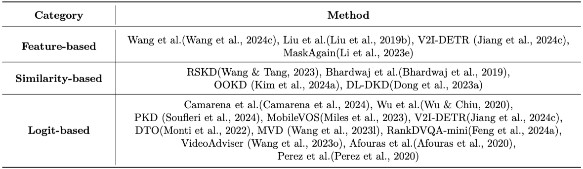
해당 논문의 Table 8

image에 temporal dimension이 추가되어 모든 frame을 무거운 model로 처리하기 비싸다.

Image/Text만큼 오래 연구되지는 않았지만 최근 적용이 증가하고 있다. Video Action Recognition, Video Classification, Video Object/Instance Segmentation, Partially Relevant Video Retrieval, Trajectory Forecasting, Masked Video Modeling 등을 다룬다. $x \rightarrow (x_1, x_2, \dots, x_T)$ Table 8에서도 method를 Feature / Similarity / Logit으로 분류하며, 3D처럼 새로운 source taxonomy가 생기는게 아니라 knowledge가 temporal information을 포함한다는 점이 달라진다.

Temporal Consistency

large video model의 complexity는 edge deployment를 어렵게 하므로 KD로 computation과 memory를 줄인다.

MobileVOS : resource-constrained device의 semi-supervised VOS를 위해 pixel-wise representation distillation을 사용하며, frame 간 feature consistency도 유지

즉 $F_t$ 하나가 아니라 $F_t, F_{t+1}$ 사이의 temporal consistency까지 중요하다.

Offline Video Teacher → Online Frame Student

Kim et al. (2024a) 는 Video Instance Segmentation에서 Teacher는 전체 video sequence를 offline으로 $T(x_1, \dots, x_T)$, Student는 real-time을 위해 각 frame을 online으로 $S(x_t)$ 처리한다. Teacher가 전체 temporal context로 얻은 similarity knowledge를 Student에 distill하여 future frame 없이도 좋은 prediction을 하게 한다.

Online Distillation for Live Video

Mullapudi et al. (2019) 는 live video에서 online feature distillation으로 low-cost semantic segmentation을 수행한다.

📌 Video → Image

V2I-DETR은 video Teacher가 여러 frame의 temporal information을 쓰고 Student는 single image를 처리한다. medical video lesion detection에서 real-time inference와 높은 detection accuracy를 동시에 추구한다. $T_{\text{Video}} \rightarrow S_{\text{Image}}$

Video → Image
Video → Text / Text → Video
Audio → Video / Video → Audio
video captioning에서 spatio-temporal graph + KD로 spurious correlation에 대한 robustness 향상

Mullapudi et al. (2019) : Online Model Distillation for Efficient Video Inference

generic high-quality model은 전체 real-world distribution을 처리하도록 만들어졌지만, 한 camera가 보는 video distribution은 훨씬 좁다. lightweight Student를 live video stream에 online으로 계속 specialize하고, Teacher는 모든 frame이 아니라 필요할 때만 간헐적으로 실행하여 새로운 supervision을 준다. Mask R-CNN Teacher에 가까운 quality를 유지하면서 runtime을 크게 줄인다. 한번 distill하고 고정하는 것이 아니라 deployment 중 들어오는 data에 맞춰 Student가 계속 Teacher에게 배운다.

Video에서 Teacher가 강한 이유
여기서도 Teacher의 우월성은 model size만이 아니다. Teacher는 미래를 포함한 더 많은 temporal context를 볼 수 있지만 Student는 현재 frame만 보고 즉시 prediction해야 한다. 즉 KD가 offline information을 online model에 전달하는 mechanism으로 작동한다. Mullapudi et al.은
1 train once → deploy 에서 Deploy → Observe → Teacher supervision → Student adaptation
이 반복되는 구조로, Section 3의 Online Distillation을 streaming application에 적용한 사례인거 같다. V2I-DETR도 Multi-view에서 본 Multi-view Teacher → Single-view Student와 같은 원리이다.
1 Multi-frame Video Teacher → Single-frame Image Student

Modalities 정리

modality가 바뀌어도 KD의 원리 전체가 바뀌는 것은 아니다. 여전히 Logit / Feature / Similarity, Offline / Online / Self, Cross-modal / Contrastive / Adaptive / Attention을 조합하며, 같은 KD primitive를 modality-specific information에 맞게 재해석한다. $\begin{aligned} \text{Image} &: \text{spatial / semantic representation} \\ \text{3D} &: \text{geometry / sensor information} \\ \text{Text} &: \text{sequence / linguistic representation} \\ \text{Speech} &: \text{acoustic / speaker / generative capability} \\ \text{Video} &: \text{temporal / multimodal context} \end{aligned}$

Section 5의 핵심
KD가 Text에도, Speech에도, Video에도 된다로 끝내면 의미가 약하다. 더 중요한 것은 Teacher가 가진 privileged information의 종류가 다양해졌다는 것인거 같다. $\begin{aligned} \text{Better Model} &\rightarrow \text{Model Capacity} \\ \text{Better Sensor} &\rightarrow \text{Geometry} \\ \text{More Views} &\rightarrow \text{Spatial Context} \\ \text{High-resource Language} &\rightarrow \text{Linguistic Knowledge} \\ \text{Offline Speech Model} &\rightarrow \text{Accurate Acoustic Context} \\ \text{Whole Video} &\rightarrow \text{Temporal Context} \end{aligned}$ Teacher는 Student보다 더 많은 useful information에 접근할 수 있는 system이고, KD는 그 information을 training 때 풍부하게 쓰면서 inference는 싸게 만드는 bridge이다.

Rich information at training → Efficient information use at inference

Section 6 : Applications

KD가 현대 AI model 안에서 어떤 역할을 맡는가?

Section 5가 어느 data에 적용하는가였다면, Section 6은 LLM, FM, SSL, Diffusion 같은 현대 AI paradigm 안에서 KD 자체가 어떤 역할을 맡게 되었는가를 다룬다.

1. Distillation in LLMs

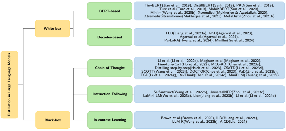
해당 논문의 Fig 8

LLM → SLM으로 압축하되, Teacher 내부에 얼마나 접근할 수 있는가가 설계 변수가 된다.

LLM은 parameter 수와 attention block 수가 매우 많아 real-time deployment가 어렵기 때문에 Small Language Model(SLM) 로 압축하는 KD가 중요하다. $T_{\text{LLM}} \rightarrow S_{\text{SLM}}$ 이때 Teacher access에 따라 사용할 수 있는 knowledge가 완전히 달라진다.

White-box : logits, hidden states, attention scores 등 내부 information에 접근 가능
Black-box : GPT-4, Gemini 같은 closed-source Teacher의 prediction/output만 이용 가능

Fig 8은 이를 아래처럼 분류한다.

White-box : BERT-based → Decoder-based
Black-box : ICL / Instruction Following / CoT

White-box : BERT based

내부에 접근할 수 있으므로 기존 KD의 source를 그대로 활용한다. → Logit + Hidden State + Attention

DistilBERT : pretrained Teacher로 pre-training 단계에서 Student를 distill하고 soft probability를 맞춤
MiniLM : Teacher 마지막 Transformer layer의 self-attention relation을 distill
MobileBERT : 별도의 Teacher를 먼저 구성한 뒤 feature와 attention transfer
TinyBERT : Logit + Attention Matrix + Hidden State + Embedding Output을 모두 사용하며, pre-training과 task-specific training 모두에서 KD 수행
PKD : intermediate layer를 이용한 incremental distillation
XtremeDistil 계열 : architecture/task dependence를 줄이는 방향

즉 BERT 시대에도 이미 Section 2의 Logit → Feature / Attention 확장이 그대로 나타난다.

White-box : Decoder based

최근 White-box KD는 autoregressive decoder LLM으로 이동하고 있다. (MetaDistill, GKD, PC-LoRA, MiniLLM, CKA, feature-dynamics alignment 등) $p(y_1, \dots, y_T | x) = \prod_t p(y_t | x, y_{<t})$ decoder LLM은 자신의 앞선 output을 다음 prediction의 context로 다시 쓰기 때문에 Student가 생성하는 sequence 자체가 training distribution과 달라지는 문제가 생긴다.

📌 GKD : Student가 직접 생성한 sequence $y \sim p_S(y x)$에 대해 Teacher feedback을 받아 학습
📌 MiniLLM : KL 방향을 뒤집은 reverse KL을 사용하여 Student가 Teacher의 low-probability region을 과대평가하는 문제를 완화 $D_{KL}(p_T \parallel p_S) \quad \rightarrow \quad D_{KL}(p_S \parallel p_T)$

📌 Industrial Pipeline

White-box KD는 academic compression에 머무르지 않고 산업에서 작은 LLM을 만드는 pre-/post-training 과정에 들어가 있다.

Large pretrained LLM → Pruning / Quantization → KD / Post-training → Compact LLM

LLM-QAT 계열 : quantized Teacher/Student와 data-free distillation 결합
NVIDIA : large Teacher를 pruning한 뒤 KD로 작은 model 복원
Gemma 3 : logit sampling
Qwen3 : weak-to-strong distillation

Black-box

closed-source LLM이 늘면서 Black-box KD가 주목받고 있다. hidden state, attention, internal logit에 접근할 수 없으므로 Teacher가 외부로 생성하는 response를 이용한다.

In-Context Learning (ICL) : Teacher가 Task Description + Few-shot Examples + Query에 대해 response를 생성하고, Student는 task knowledge와 in-context example을 해석하는 능력을 학습
- ILD : ICL objective + language modeling objective 결합
- AICD : ICL과 reasoning을 동시에 distill
- LLM-R : Teacher에게 좋은 in-context example을 주기 위한 retriever를 반복적으로 학습
Instruction Following (IF) : zero-shot capability 향상이 목적이며, Teacher가 instruction과 input/output example을 생성하고 Student가 그 synthetic data로 fine-tuning
- Self-Instruct : Instruction + Input + Output을 생성하고 invalid example을 filtering한 뒤 fine-tuning
- UniversalNER : 특정 application class를 위한 instruction tuning
- Lion : Student에게 어려운 instruction을 adversarial하게 생성
- LaMini-LM : 대규모 instruction dataset 구축
📌 Chain-of-Thought (CoT) : Black-box에서 가장 popular한 category이다. Teacher가 final answer뿐만 아니라 rationale을 함께 생성하고 Student가 이를 학습한다. $x \rightarrow \underbrace{r_1 \rightarrow r_2 \rightarrow \cdots \rightarrow r_K}_{\text{Teacher rationale}} \rightarrow y$
- Magister et al. : model size와 dataset size의 trade off를 분석하며 reasoning을 smaller model에 전달
- MCC-KD : 하나의 sample에 여러 reasoning $r^{(1)}, \dots, r^{(M)}$을 생성하고 consistency와 diversity를 함께 고려
- Distilling Step-by-Step : rationale을 추가 supervision으로 쓰고 label과 rationale을 multi-task로 학습
- TDG : 정답이 틀린 reasoning을 버리지 않고 positive + negative reasoning 모두 활용
- RevThink : forward reasoning뿐만 아니라 backward question/reasoning까지 생성하여 양방향 학습

Single correct rationale → Multiple / Positive + Negative / Forward + Backward reasoning

두 방식의 장단점을 저자들은 직접 비교한다.

White-box : richer knowledge로 더 효과적인 transfer가 가능하지만, training 동안 큰 Teacher를 직접 써야 해서 computational cost가 높고, closed-source Teacher에는 적용 자체가 불가능
Black-box : output만 얻으면 되므로 Teacher 접근성이 훨씬 높지만, Student가 배우는 것은 결국 Teacher가 생성한 finite dataset이라 Teacher의 모든 behavior를 포괄하지 못해 generalizability가 낮을 수 있음

저자들은 둘을 결합하는 two-stage strategy도 제안한다. $T_{\text{closed}} \xrightarrow{\text{Black-box}} T_{\text{open}} \xrightarrow{\text{White-box}} S$

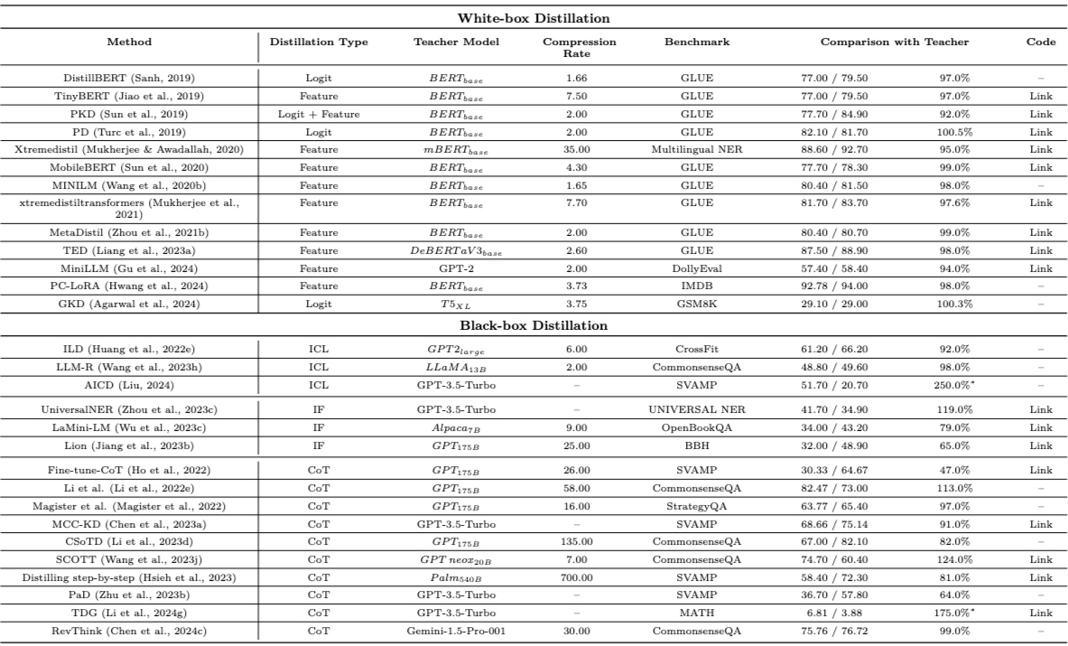
해당 논문의 Table 16

Table 16에서 White-box와 Black-box를 따로 비교하지만, 연구마다 Teacher, Student, dataset, benchmark(GLUE, GSM8K, CommonsenseQA, SVAMP, BBH, MATH 등)가 크게 달라 완전한 fair comparison은 어렵다. 저자들은 이 표를 근거로 LLM에서는 높은 compression rate로 줄이면서 Teacher에 가까운 성능을 유지할 수 있어 KD가 특히 중요하다고 평가한다. 단, * 표시 row는 Teacher-Student 비교가 아니라 Student의 distillation 전/후 비교이다.

Sanh et al. (2019) : DistilBERT

기존 KD는 주로 downstream task별 Student compression에 집중했다. DistilBERT는 BERT의 pre-training 단계 자체에서 distill하며 language modeling loss, distillation loss, cosine distance loss를 결합한다. 약 40% 작고 약 60% 빠르면서 language understanding capability의 약 97%를 유지한다고 보고한다. Task-specific Student → General-purpose pretrained Student로, KD가 pretrained model을 만드는 과정에 들어간 초기 사례이다.

Agarwal et al. (2024) : GKD

autoregressive model에서는 training 때 본 sequence와 inference에서 Student가 실제로 생성하는 sequence가 달라지는 train-inference distribution mismatch가 생긴다. Student가 $\hat{y} \sim p_S(\cdot|x)$를 직접 생성하고 그 sequence에 대한 Teacher feedback으로 학습하는 on-policy distillation을 사용하며, 다양한 divergence objective를 선택할 수 있다. Teacher가 제공한 정답만 학습 → Student가 실제로 저지르는 실수에서 학습

Gu et al. (2024) : MiniLLM

low-capacity Student는 Teacher의 generation distribution을 완벽하게 표현할 수 없고, forward KL은 Teacher의 low-probability 영역까지 과도하게 덮으려 한다. reverse KL $D_{KL}(p_S \parallel p_T)$를 사용하여 Student 자신의 distribution에서 sequence를 생성하고 Teacher가 선호하는 major mode에 집중하게 한다. Teacher distribution 전체를 복제하는 대신 Student capacity 안에서 Teacher의 중요한 mode를 학습한다. → Adaptive KD에서 본 capacity gap 문제가 LLM에서 다시 나타난 것

Wang et al. (2022) : Self-Instruct

instruction-following model에는 많은 human-written instruction이 필요하지만 양과 다양성에 한계가 있다. language model이 스스로 instruction, input, output을 생성하고 중복/부적절한 sample을 filtering한 뒤 fine-tuning한다. 엄밀히는 하나의 LM이 자신의 generation을 bootstrap하는 framework에 가깝지만, survey는 Black-box IF distillation의 대표 흐름으로 포함한다. Human instruction annotation → Model-generated supervision

Hsieh et al. (2023) : Distilling Step-by-Step

기존 fine-tuning이나 LLM label distillation으로는 작은 model이 large LLM 수준에 도달하려면 많은 data가 필요하다. Teacher에서 final label뿐만 아니라 rationale을 추가 supervision으로 추출하고, Student를 label prediction과 rationale 관련 task의 multi-task framework로 학습한다. Answer only → Answer + Rationale로, hidden state를 볼 수 없어도 Teacher가 외부로 표현한 rationale을 observable intermediate knowledge로 쓸 수 있다.

LLM에서 바뀐 것
Teacher가 커진것 뿐만 아니라 Teacher access 자체가 KD 설계 변수가 되었다. → Teacher capability + Teacher accessibility White / Black은 우열이 아니라 trade off로 보는것이 맞는거 같다. $\text{Knowledge Richness} \leftrightarrow \text{Teacher Accessibility}$ 또한 Decoder LLM에서는 generation dynamics가 KD 설계에 들어온다. BERT에서는 어느 hidden state/attention을 맞출지가 문제였다면, 이제는 Student가 실제 inference 때 방문하는 sequence에서도 Teacher knowledge를 받을 수 있는가가 문제이다. KD의 위치도 바뀌었다.
1 Model을 완성 → 마지막에 KD로 압축 에서 KD가 model family를 구축하는 training pipeline 안으로

CoT와 Feature KD의 평행 관계
Future Direction에서 본 CoT Distillation이 여기서 구체적으로 나타난다.
1 2 전통적인 DNN : Final Logit → Intermediate Feature Closed LLM : Final Answer → Externally generated intermediate rationale
기술적으로 같은 것은 아니지만 final output만으로는 supervision이 부족하므로 intermediate information을 더 제공한다는 문제의식은 같다. LLM KD의 대상은 아래처럼 넓어졌다고 볼 수 있다. (survey가 직접 선언한 chronology는 아니고 흐름 중심의 해석이다) $\text{Probability} \rightarrow \text{Representation} \rightarrow \text{Generated Sequence} \rightarrow \text{Instruction / Reasoning Behavior}$

Teacher prediction을 따라하는 compression → generation behavior와 reasoning까지 전달하는 capability transfer

2. Foundation Model Distillation

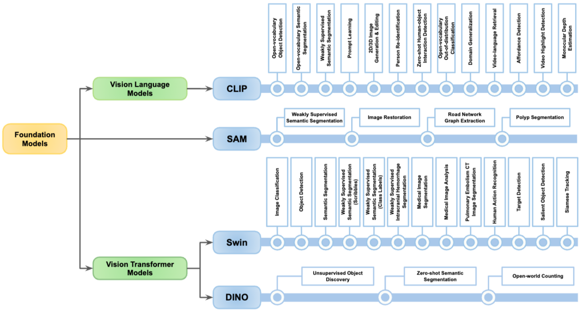
해당 논문의 Fig 9

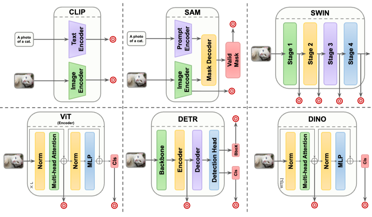
해당 논문의 Fig 10

특정 task의 prediction이 아니라 범용 pretrained representation / capability를 전달한다.

FM은 여러 downstream task에 generalize하도록 대규모로 pretraining되었지만 model size와 computational cost가 커서 배포가 어렵다. 따라서 FM의 knowledge를 smaller, task-specific, efficient Student로 옮긴다. knowledge source로 CLIP, ChatGPT, DALL-E, SAM, DINO, ViT / DETR / Swin 등을 언급한다.

Fig 9 : FM의 knowledge가 어느 task로 distill되는지 정리 (CLIP → open-vocabulary detection/segmentation, WSSS, prompt learning, generation/editing, domain generalization, video-language retrieval, depth estimation 등)
Fig 10 : CLIP의 image/text encoder, SAM의 image/prompt encoder와 mask decoder, ViT/Swin/DETR/DINO의 architecture를 나란히 보여주며 어느 representation에서 knowledge를 추출할 수 있는가를 시각화

즉 FM distillation에서는 final logit보다 encoder feature / embedding / attention / semantic representation이 중요한 source가 된다.

1. Vision-Language Model

VLM은 visual과 textual data를 joint representation space에서 연결하며, 대부분 CLIP 중심으로 전개된다. $f_I(x) \leftrightarrow f_T(t)$ 따라서 distill할 knowledge는 Visual Feature + Text Feature + Image-Text Alignment이다.

📌 Open-vocabulary Tasks : 기존 recognition은 predefined class set $\mathcal{C} = {\text{car}, \text{person}, \dots}$에 묶여 있다. CLIP의 semantic knowledge를 detector/segmenter에 전달하면 annotation되지 않은 category까지 다룰 수 있다. detection은 global vision-language knowledge를 detector에, segmentation은 image-level CLIP knowledge를 pixel-level dense task로 가져오는 것이 문제이다.
Weakly Supervised Semantic Segmentation : class 이름의 text embedding과 CLIP image feature를 비교해 coarse class activation map을 만들고, 이를 pseudo-label로 segmentation model을 학습해 pixel annotation 의존성을 줄인다. (Future Direction에서 본 WSSS 예시)
Prompt Learning : hard prompt a photo of a [CLASS] 대신 learnable $[p_1, \dots, p_k, \text{CLASS}]$를 최적화한다. 모든 method가 좁은 의미의 Teacher→Student KD는 아니고, FM knowledge 활용이라는 넓은 문맥에서 다룬다.
Generation / Editing : CLIP의 text-image alignment로 2D/3D의 text-guided manipulation
기타 : Person Re-ID, Zero-shot HOI, Open-vocabulary OOD, Domain Generalization, Video-Language Retrieval, Affordance Detection, Video Highlight Detection, Monocular Depth Estimation

CLIP 자체를 작게 만드는 방향(TinyCLIP 등)도 있다.

2. Segment Anything (SAM)

SAM은 Image Encoder + Prompt Encoder + Mask Decoder로 구성된 general-purpose segmentation model이다. SAM의 capability를 smaller/task-specific model에 distill하면 limited annotation, limited computation, domain constraint 상황에서도 활용할 수 있다.

Lightweight SAM : 주된 bottleneck은 큰 image encoder이므로 Heavy SAM Image Encoder → Lightweight Encoder를 distill하고 prompt encoder/mask decoder와 연결
- MobileSAM : ViT-H encoder → TinyViT로 decoupled distillation
- EfficientViT-SAM : ViT-H encoder → EfficientViT로 KD 후 SA-1B에서 end-to-end training, prompt encoder와 mask decoder는 유지
SAM for WSSS : image-level tag, point, box 같은 약한 supervision으로도 좋은 mask를 만들 수 있어 high-quality pseudo-label generator로 사용
1 Weak Label → SAM → Pseudo Mask → Segmentation Student

📌 3. Multi-model Applications

여러 FM의 complementary capability를 하나의 model에 결합한다. Section 4의 Multi Teacher가 FM 수준으로 확장된 것이다.

SAM + CLIP : spatial segmentation knowledge + semantic understanding
DINO + CLIP : self-supervised visual representation + vision-language alignment
DETR + CLIP : detection capability + text semantic → open-vocabulary detection
SAM + Grounding DINO : detection/localization + segmentation
AM-RADIO (Ranzinger et al. (2024)) : CLIP, DINOv2, SAM처럼 서로 다른 objective로 학습된 VFM을 multi-teacher distillation으로 하나의 model에 통합
Theia (Shang et al. (2024)) : 여러 off-the-shelf VFM representation을 하나의 model에 distill하여 robot learning에 활용

4. Vision Transformers

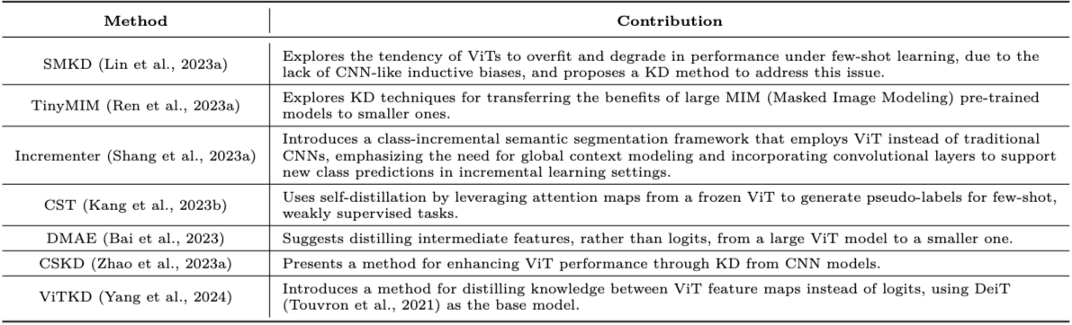
해당 논문의 Table 9

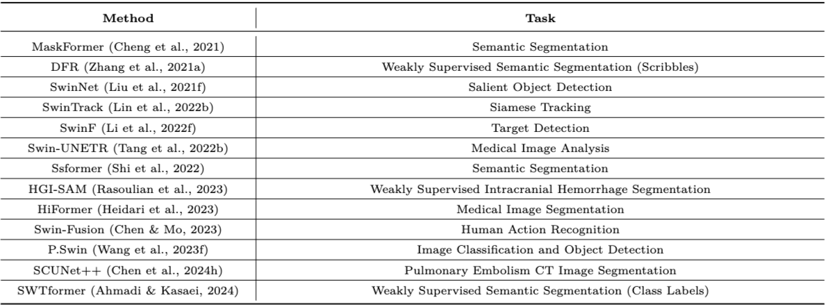
해당 논문의 Table 10

ViT는 long-range dependency와 global context를 잘 modeling하지만 large ViT는 비싸다.

ViT (Table 9)
- SMKD : inductive bias가 부족한 ViT의 few-shot overfitting 문제를 KD로 해결
- TinyMIM : large MIM pretrained model → 작은 ViT
- CST : frozen ViT의 attention map을 pseudo-label처럼 쓰는 self-distillation
- DMAE : large ViT의 intermediate feature를 작은 model로
- CSKD : CNN knowledge → ViT (같은 architecture family일 필요 없음)
- 📌 ViTKD : ViT 사이에서 intermediate feature distillation을 어떻게 할 것인가
DINO : unlabeled data에서 strong visual representation을 학습한 self-supervised ViT로, feature가 object structure를 잘 포착하여 unsupervised object discovery, open-world counting, zero-shot segmentation 등의 source가 됨. knowledge가 human-labeled prediction이 아니라 self-supervised representation이다.
DETR : detection을 end-to-end set prediction으로 구성하지만 model size가 커서 Strong DETR Teacher → Efficient Detector로 압축하며, class logit뿐만 아니라 query/object representation과 detection structure도 고려
Swin Transformer (Table 10) : hierarchical design + shifted-window attention. semantic segmentation, WSSS, salient object detection, tracking, detection, medical, action recognition, classification 등에서 encoder knowledge로 활용

FM Distillation은 실제로 세 형태가 있다.

FM 자체를 압축 : CLIP / SAM / Large ViT → Small CLIP / SAM / ViT
FM → Downstream Task : CLIP → Open-vocabulary Detector, SAM → WSSS, DINO → Object Discovery
Multiple FM → Unified Model : CLIP + SAM + DINO → S

또한 FM의 rich representation을 그대로 쓰지 않고 여러 alignment가 반복된다.

CLIP → region / text embedding alignment
TinyCLIP → cross-modal affinity alignment
ViT → layer-specific feature alignment
Multi-model → 서로 다른 Teacher representation의 aggregation

Discussion에서도 Teacher-Student architecture/capacity gap이 FM에서 특히 심각하다고 지적한다.

Gu et al. (2021) : ViLD

detector가 다룰 category를 늘리려면 새 class마다 bounding box annotation이 필요해 매우 비싸다. pretrained VLM Teacher가 category text와 object proposal region을 embedding하고, Student detector가 자신의 region embedding을 Teacher의 image/text embedding과 align한다. 이를 통해 annotation에 없는 category도 text embedding으로 일반화한다. $\text{VLM semantic space} \rightarrow \text{Detector region representation}$ 큰 detector → 작은 detector가 아니라 범용 semantic Teacher → task-specific detector로, closed vocabulary라는 task limitation을 깨는 데 KD를 쓴다.

Wu et al. (2023) : TinyCLIP

CLIP은 zero-shot representation이 뛰어나지만 large encoder 때문에 배포가 어렵다. Affinity Mimicking으로 Teacher의 cross-modal image-text alignment를 따라가게 하고, Weight Inheritance로 pretrained Teacher parameter를 효율적으로 전달하며, extreme compression에서는 progressive multi-stage distillation을 쓴다. $F_I^T \approx F_I^S \quad \rightarrow \quad \text{Relation}(I, T)_T \approx \text{Relation}(I, T)_S$ FM의 useful knowledge가 하나의 modality feature보다 cross-modal relationship 자체에 있을 수 있다.

Zhang et al. (2023) : MobileSAM

original SAM은 거대한 ViT-H encoder 때문에 mobile/edge 배포가 어렵다. SAM 전체를 재학습하지 않고 image encoder만 분리해서 TinyViT로 decoupled distillation하며, 기존 mask decoder와 호환되도록 학습한다. FM 전체를 복제하지 않고 가장 비싼 component의 reusable representation만 선택적으로 distill한다.

Wang et al. (2024) : SAM-CLIP

CLIP은 semantic understanding이 강하지만 dense localization에 한계가 있고, SAM은 localization이 강하지만 language semantic이 없다. multi-task distillation으로 두 FM의 capability를 하나의 unified backbone에 통합한다. Multi Teacher의 목표가 ensemble compression에서 서로 다른 FM의 capability composition으로 확장된 사례이다.

Ren et al. (2023) : TinyMIM

MIM은 large ViT에서는 효과적이지만 작은 ViT에서는 benefit이 제한된다. 여러 distillation target을 실험한 결과 CLS token이나 raw feature보다 token relation distillation이 효과적이고, Teacher와 Student depth가 다르면 마지막 layer보다 intermediate Teacher layer가 더 좋다고 보고한다. 좋은 foundation pretraining이 small model에 자동으로 이전되지 않으므로 KD가 bridge가 된다.

Yang et al. (2024) : ViTKD

CNN에 효과적이던 feature KD를 ViT에 그대로 쓰면 structural difference 때문에 잘 동작하지 않거나 성능이 떨어질 수 있다. ViT의 layer 특성을 분석해 shallow layer는 mimic, deep layer는 generation/reconstruction 방식처럼 layer마다 다른 전략을 쓴다. Section 2의 architectural gap과 representation alignment 문제가 ViT에서 다시 등장한다.

기존 Teacher와 FM Teacher의 차이
기존 Teacher는 이 task를 Student보다 잘 푼다는 이유로 Teacher였다면, FM은 특정 task를 넘어 재사용 가능한 representation을 이미 학습했다는 이유로 Teacher가 된다. $\underbrace{T_{\text{Task A}} \rightarrow S_{\text{Task A}}}_{\text{기존}} \quad \rightarrow \quad \underbrace{T_{\text{General}} \rightarrow S_{\text{Task A}}}_{\text{FM}}$ 그래서 질문이 Teacher prediction을 어떻게 복사할까?에서 범용 representation 중 downstream task에 필요한 부분을 어떻게 추출하고 옮길까? 로 바뀐거 같다. Open-vocabulary는 KD가 Student의 semantic scope 자체를 넓히는 도구가 된 것이고, WSSS에서는 FM이 pseudo-supervision generator로 쓰인다. 3D에서 2D FM을 point cloud로 옮기던 흐름과도 같다. 또한 FM Teacher에도 종류가 있어서, Teacher는 accuracy가 아니라 어떤 종류의 knowledge가 필요한가로 선택하게 된다.
1 2 3 CLIP : What is it? → language-aligned semantic knowledge SAM : Where exactly is it? → spatial segmentation knowledge DINO : self-supervised visual structure

FM 시대의 역설
Teacher가 강해질수록 전달 가능한 knowledge는 많아지지만 Teacher-Student representation gap도 커진다. 그래서 더 좋은 Teacher를 찾는 것만이 아니라 그 knowledge를 Student가 쓸 수 있는 representation으로 어떻게 번역할 것인가가 중요하다. Feature Transformation, Adaptive KD, Contrastive KD가 FM distillation과 만나는 이유가 여기 있다. 또 여러 FM이 존재하는 지금은 질문이
1 어떻게 이 Teacher를 distill할까? → 어느 FM의 어떤 capability를 이 Student에게 가져올 것인가?
로 바뀌고, Knowledge Distillation → Knowledge Amalgamation / Capability Composition으로 확장되는거 같다.

Task-specific expert → General-purpose knowledge repository / Compression + Downstream Knowledge Transfer + Capability Composition

3. Distillation in Self-supervised Learning

teacher-student 구조 자체가 label 없이 representation을 학습하는 training mechanism이 된다.

SSL은 human label 없이 representation을 학습하며, 저자들은 computer vision의 여러 prominent SSL 방법이 self-distillation과 밀접하게 연결되어 있다고 본다. label 대신 같은 image의 서로 다른 augmentation을 만들고 두 representation이 같은 semantic을 나타내도록 학습한다. $x \xrightarrow{a_1} x^{(1)}, \qquad x \xrightarrow{a_2} x^{(2)}$ 즉 different views of the same data 사이의 consistency가 supervision 역할을 한다.

SimCLR → MoCo → BYOL

SimCLR (Chen et al. (2020c)) : 하나의 shared network에 같은 image의 서로 다른 augmentation을 넣고 두 embedding의 consistency를 학습
MoCo / BYOL : Student는 backpropagation으로 학습하고 Teacher 측은 Student의 EMA로 update $\theta_T \leftarrow m\theta_T + (1-m)\theta_S$ Teacher가 Student를 천천히 따라오므로 Student보다 안정적인 representation을 제공한다.
BYOL은 두 view를 각각 Student(online)와 Teacher(target)가 처리하고, Student가 Teacher representation을 예측하도록 학습한다.

원 논문 기준으로 구분해야 하는 부분
survey는 SimCLR부터 self-distillation 흐름에 가깝게 묶지만, 원 논문 기준으로는 구분하는 것이 정확하다.
SimCLR : 같은 image의 augmented view는 positive, batch의 다른 image는 negative / EMA branch 없음 → Contrastive SSL
MoCo : query encoder와 momentum key encoder, queue에 저장한 과거 key로 크고 일관된 contrastive dictionary 구축 → Momentum Contrastive SSL
BYOL : online → target representation 예측, negative 없음, EMA target → EMA Target based SSL
DINO : 저자들이 직접 self-distillation with no labels라고 정의 → 명시적 Self Distillation
따라서 SimCLR부터 모두 self-distillation이라고 정리하지 않는 것이 맞다.

Prototype Assignment

Caron et al. (2020) 은 여러 prototype을 만들고 같은 image의 augmentation이 동일한 prototype assignment를 예측하도록 학습한다. representation target이 raw embedding에서 latent cluster / prototype structure까지 확장된다. survey 본문은 SwAP이라고 적었지만 인용된 method는 SwAV (Swapping Assignments between Views) 이다.

📌 DINO / DINOv2

같은 image에서 global crop과 local crop을 만들어 유사한 Teacher/Student network에 넣고, Teacher는 EMA로 update하며 두 representation이 유사해지도록 학습한다. 저자들은 이러한 local-to-global learning이 segmentation에 적합한 representation을 만든다고 설명한다. $\text{Local Student View} \rightarrow \text{Global Teacher Target}$ DINOv2는 DINO의 단순 scale-up이 아니다.

class token에 대한 DINO loss (image-level self-distillation) + masking한 Student patch로 Teacher patch representation을 예측하는 iBOT loss (patch-level masked learning) + KoLeo regularizer
📌 작은 architecture는 처음부터 학습하지 않고 frozen large ViT-g에서 distill

즉 DINOv2 안에는 두 종류의 distillation이 함께 있다.

SSL training : EMA Teacher → Student
Model scaling : Large frozen ViT-g → Small ViT

이후 확장

BINGO : pretrained SSL model로 image를 bag 단위로 grouping하고 intra-sample과 inter-sample loss를 함께 최소화
Wang et al. (2023l) : image SSL Teacher의 spatial feature와 video SSL Teacher의 spatio-temporal feature를 하나의 Student에 전달
Song et al. (2023a) : 여러 parallel SSL process 사이에 consistency loss 추가
Gao et al. (2022c) : 기존 KD approach를 SSL framework에 통합하고 SSL-pretrained Teacher 활용

Instance → Bag / Dataset Relation → Multiple SSL Teachers → Spatial + Temporal Knowledge

SSL Teacher → Small Student

large model은 SSL의 benefit을 잘 받지만 small model은 같은 objective를 직접 학습해도 representation quality가 충분하지 않다는 관찰에서 출발한다. 따라서 강한 SSL model을 먼저 학습한 뒤 작은 Student로 distill한다. (CompRess, SEED, SimReg, ISD, Dadashzadeh et al.)

CompRess : similarity-based distillation으로 strong SSL Teacher의 knowledge 전달
SEED : sample queue의 anchor와의 distance 관계를 Teacher와 맞춤 $D_T(i,j) = D(F_T(x_i), A_j), \quad D_S(i,j) = D(F_S(x_i), A_j), \qquad D_S \approx D_T$
Navaneet et al. (2022) : Student representation 뒤에 MLP projector를 추가하는 효과를 보임 → $F_T \approx g(F_S)$처럼 projection space에서 matching

Section 6.3에는 목적이 다른 두 흐름이 섞여 있다.

A. KD as a Learning Mechanism : No Labels → Self-generated Teacher Target → Representation Learning (MoCo / BYOL / DINO)
B. KD as Representation Compression : Strong SSL Teacher → Small Student (CompRess / SEED / SimReg)

Contrastive Learning과 Self Distillation도 서로 배타적이지 않다. Contrastive는 positive는 가깝게, negative는 멀게이고 Self Distillation은 Teacher/Target representation을 Student의 supervision으로 사용하는 것이므로 함께 쓸 수도 있고, BYOL/DINO처럼 negative 없이 self-distillation target만 쓸 수도 있다.

Grill et al. (2020) : BYOL

기존 contrastive SSL은 collapse를 막기 위해 많은 negative가 필요해 large batch나 memory bank가 필요했다. online network $f_\theta$와 target network $f_\xi$를 사용하고, online은 target representation을 예측하도록 gradient로 학습하며 target은 $\xi \leftarrow \tau\xi + (1-\tau)\theta$로 update한다. negative pair 없이 학습한다. Teacher가 external pretrained model이 아니라 Student 자신의 EMA version이 되는 self-distillation 구조를 명확하게 보여준다.

Caron et al. (2021) : DINO

self-supervised pretraining이 ViT에 어떤 representation을 만드는지 탐색한다. 저자들이 직접 self-distillation with no labels로 정의하며, 같은 architecture의 Student와 EMA Teacher, multi-crop augmentation으로 Teacher prediction과 Student의 다른 view prediction을 맞춘다. label과 negative 없이 학습되며, self-supervised ViT의 attention에서 object boundary와 semantic segmentation structure가 자연스럽게 나타난다고 보고한다. KD가 compression에서 완전히 벗어나 representation learning objective 자체가 된 대표 사례이다.

Oquab et al. (2023) : DINOv2

image-level DINO loss와 patch-level iBOT loss를 결합하고 Teacher는 EMA로 update한다. 또한 작은 model은 large ViT-g를 frozen Teacher로 두고 distill한다. 하나의 method 안에 learning mechanism으로서의 KD와 compression으로서의 KD가 공존한다.

Abbasi Koohpayegani et al. (2020) : CompRess

large network에서는 SSL representation이 강해졌지만 small network는 같은 방법으로 그 benefit을 얻지 못했다. feature vector를 복사하는 대신 memory bank의 data point들과 이루는 relative similarity distribution을 맞춘다. $q_T(\cdot|x) \approx q_S(\cdot|x)$ 작은 AlexNet의 SSL representation이 당시 supervised AlexNet baseline을 넘는 결과도 보고한다. Small model이 SSL을 처음부터 잘 학습하게 만드는 대신 large SSL model이 배운 geometry를 압축한다.

SSL에서 Teacher의 의미
기존 KD에서는 Teacher가 이런 prediction을 해야 한다는 supervision을 줬다면, SSL에서는 같은 object의 다른 view라면 representation도 일관되어야 한다는 supervision이 된다. 그 target을 다른 branch, EMA model이 제공하기 시작하면서 자연스럽게 self-distillation 형태가 되는거 같다. $\underbrace{T_{\text{already strong}} \rightarrow S}_{\text{기존}} \quad \rightarrow \quad \underbrace{T_t = \text{EMA}(S_{0:t})}_{\text{BYOL / DINO}}$ Teacher는 이미 정답을 아는 expert가 아니라 Student에게 안정적인 target을 제공하는 mechanism으로 재해석된다. Section 3에서 본 Teacher의 확장이 가장 강하게 나타나는 부분이다. 흐름도 단순 chronology보다
1 2 Cross-view SSL → Slow target representation → Explicit self-distillation 좋은 negative를 어떻게 만들까? → negative 없이도 안정적인 target을 스스로 만들 수 있는가?
로 보는게 정확한거 같다. 한편 CompRess, SEED를 보면 SSL representation distillation에서는 $F_T \approx F_S$보다 $\text{Relation}(F_T) \approx \text{Relation}(F_S)$가 자연스럽다. capacity가 달라 raw representation은 달라도 data 사이의 semantic geometry는 유지할 수 있기 때문이다.

먼저 학습된 큰 model → 학습 중 스스로 만들어내는 안정적인 target

4. Diffusion Distillation

model size보다 iterative denoising이라는 sampling process 자체가 bottleneck이다.

diffusion은 image, text, 3D에서 generation quality가 높지만 iterative denoising 때문에 inference가 비싸다. $x_T \rightarrow x_{T-1} \rightarrow \cdots \rightarrow x_1 \rightarrow x_0$ 하나의 output에 수십~수백번 이상의 forward가 필요할 수 있으므로 efficiency bottleneck은 Model Size + Number of Sampling Steps이다. 저자들은 Teacher의 soft output이나 internal representation을 전달하면서 훨씬 적은 sampling step으로 비슷한 quality를 얻는 것을 핵심 목표로 설명한다. 네 방향으로 정리한다.

Feature-level
Sampling Process
Adversarial / Data-Free
Consistency Models

1. Feature-level

Student가 Teacher의 internal representation $F_T(x_t, t)$를 mimic하여 convergence와 sampling efficiency를 개선한다.

denoising을 이용한 feature alignment
external guidance를 이용한 feature transfer
cross-sample consistency
feature distillation + model compression

Section 4에서 본 DiffKD(Student feature를 Teacher feature의 noisy version으로 보고 denoise)도 다시 언급된다. 기존 Feature KD를 diffusion representation에 적용한 쪽에 가깝다.

📌 2. Sampling Process

Teacher가 여러 step에 걸쳐 수행하던 transition을 Student가 더 적은 step으로 수행한다. $x_t \rightarrow x_{t-1} \rightarrow x_{t-2} \quad \Rightarrow \quad x_t \rightarrow x_{t-2}$

Progressive Distillation (Salimans & Ho (2022)) : Teacher의 2 step을 Student의 1 step으로 합치고, 이를 반복하여 $N \rightarrow \frac{N}{2} \rightarrow \frac{N}{4} \rightarrow \cdots$로 줄인다. 다만 여러 세대의 Student를 순차적으로 만들어야 해서 training이 cumbersome하다.
1 Inference Cost ↓ ↔︎ Distillation Training Complexity ↑
Distribution Matching Distillation (Yin et al. (2024c)) : 점진적으로 줄이는 대신 multi-step Teacher의 전체 output distribution을 one-step Student가 직접 맞춘다. point-wise output이 아니라 distribution 전체를 맞추는 것이 핵심이다. $p_S(x) \approx p_T(x)$

3. Adversarial / Data-Free

Adversarial (Sauer et al. (2024), Mekonnen et al. (2024)) : discriminator가 Teacher sample과 Student sample을 구별하고 Student는 구별되지 않도록 학습하여 $p_S(x) \approx p_T(x)$를 강제한다. few/one-step generation이 가능하지만 training instability가 있을 수 있다.
Data-Free (EM Distillation) : large synthetic dataset이나 original data 없이 연속된 denoising step 사이에서 bootstrap하여 Student를 학습한다.

4. Consistency Models

diffusion trajectory에서 서로 다른 noise level의 point들이 같은 final clean sample로 mapping되도록 학습한다. $f(x_t, t) \approx x_0 \quad (\forall t)$ 따라서 $x_T \xrightarrow{f} x_0$의 one-step generation이 가능하고, 필요하면 multiple step으로 quality와 compute를 조절할 수 있다. (original, Improved, latent-space variants, stability/scalability improvement) low-latency generation이 가능하지만 적절한 calibration이 없으면 quality collapse가 생길 수 있다.

Consistency Model ≠ 항상 KD
원 논문은 두 경우를 구분한다.
1 2 Pretrained Diffusion Teacher 사용 → Consistency Distillation Data에서 직접 학습 → Consistency Training
후속 Improved Techniques는 아예 Teacher 없이 직접 학습하는 방향을 개선한다. 즉 consistency라는 model principle이 있고, 이를 Teacher diffusion에서 학습시킬 때 KD가 들어가는 것이다.

DreamFusion, ProlificDreamer : pretrained text-to-image diffusion의 knowledge로 3D representation을 optimize → 2D Generative FM → 3D Generation
Diff-Instruct : pretrained diffusion의 knowledge를 여러 task/model로 transfer하는 general framework

네 방향의 trade off는

Sampling Process : 매우 큰 acceleration ↔︎ quality 유지와 training complexity
Adversarial / Data-Free : flexibility ↔︎ training stability
Consistency : 매우 낮은 latency ↔︎ calibration과 stable training

결국 Diffusion Distillation 전체가 Generation Speed ↔︎ Generation Quality를 다룬다.

Teacher가 제공하는 knowledge의 단위도 방향마다 다르다.

Feature-level : $K_T = F_T$
Sampling Process : $K_T = \text{multi-step transition}$
Distribution Matching : $K_T = p_T(x)$
Consistency Distillation : $K_T = \text{trajectory endpoint consistency}$
Text-to-3D : $K_T = \text{score / generative prior}$

Salimans & Ho (2022) : Progressive Distillation

diffusion은 좋은 quality를 위해 수백~수천번의 evaluation이 필요하다. 학습된 deterministic sampler의 두 step 결과를 한번에 예측하는 Student를 학습하고, Student를 다시 Teacher로 삼아 $T^{(N)} \rightarrow S^{(N/2)}$를 반복한다. 8192-step에서 4-step까지 줄이면서 perceptual quality를 상당 부분 유지한다고 보고한다. Teacher의 prediction이 아니라 Teacher가 여러 단계에 걸쳐 수행한 computation의 결과를 한번의 transition으로 압축한다.

Yin et al. (2024) : DMD

progressive distillation도 반복적인 과정이 필요하다. one-step generator의 distribution과 Teacher diffusion distribution 사이의 approximate KL을 최소화하며, gradient를 target distribution과 Student synthetic distribution의 두 score function 차이 $s_{\text{real}}(x) - s_{\text{fake}}(x)$로 구성한다. 여기에 Teacher multi-step output의 large-scale structure를 맞추는 regression loss를 함께 쓴다. ImageNet $64 \times 64$에서 FID 2.62를 보고한다. Teacher trajectory의 각 step이 아니라 Teacher가 최종적으로 만드는 distribution 자체를 학습한다.

Song et al. (2023) : Consistency Models

같은 probability-flow trajectory 위의 서로 다른 point를 같은 clean endpoint로 mapping하는 consistency function을 학습하여 one-step과 few-step sampling을 모두 지원한다. pretrained diffusion Teacher에서 distill(Consistency Distillation)할 수도, data에서 직접 학습(Consistency Training)할 수도 있다. 여러 denoising step을 어떻게 줄일까? 가 아니라 처음부터 모든 noise level에서 같은 endpoint를 직접 예측하는 model을 만들자로 문제를 재구성한다.

Diffusion이 KD에 가져온 변화
Student가 Teacher보다 반드시 작을 필요가 없다. 기존이 Large Model → Small Model이었다면 여기서는
1 Long Generation Process → Short Generation Process
자체가 distillation 대상이다. Future Direction에서 본 Diffusion → sampling step reduction이 이것이고, Parallel WaveNet과 같은 큰 흐름인거 같다. 발전 방향은
1 Teacher 내부 feature를 따라감 → 여러 sampling step을 압축 → 최종 distribution을 직접 맞춤 → direct mapping이 가능한 model principle로 재구성
으로 step-level imitation에서 function / distribution-level transfer로 abstraction level이 올라가는 것이다. knowledge의 단위도 output/feature에서 trajectory + distribution + generative dynamics로 넓어졌다. 또한 Adversarial 방식은 Section 4의 Discriminator in the Loop가, Data-Free 방식은 Teacher가 data generator 역할까지 하는 LLM Black-box KD와 비슷한 흐름이 다시 나타난 것이다.

Model Compression → Computation / Generation Process Distillation

5. Visual Recognition Distillation

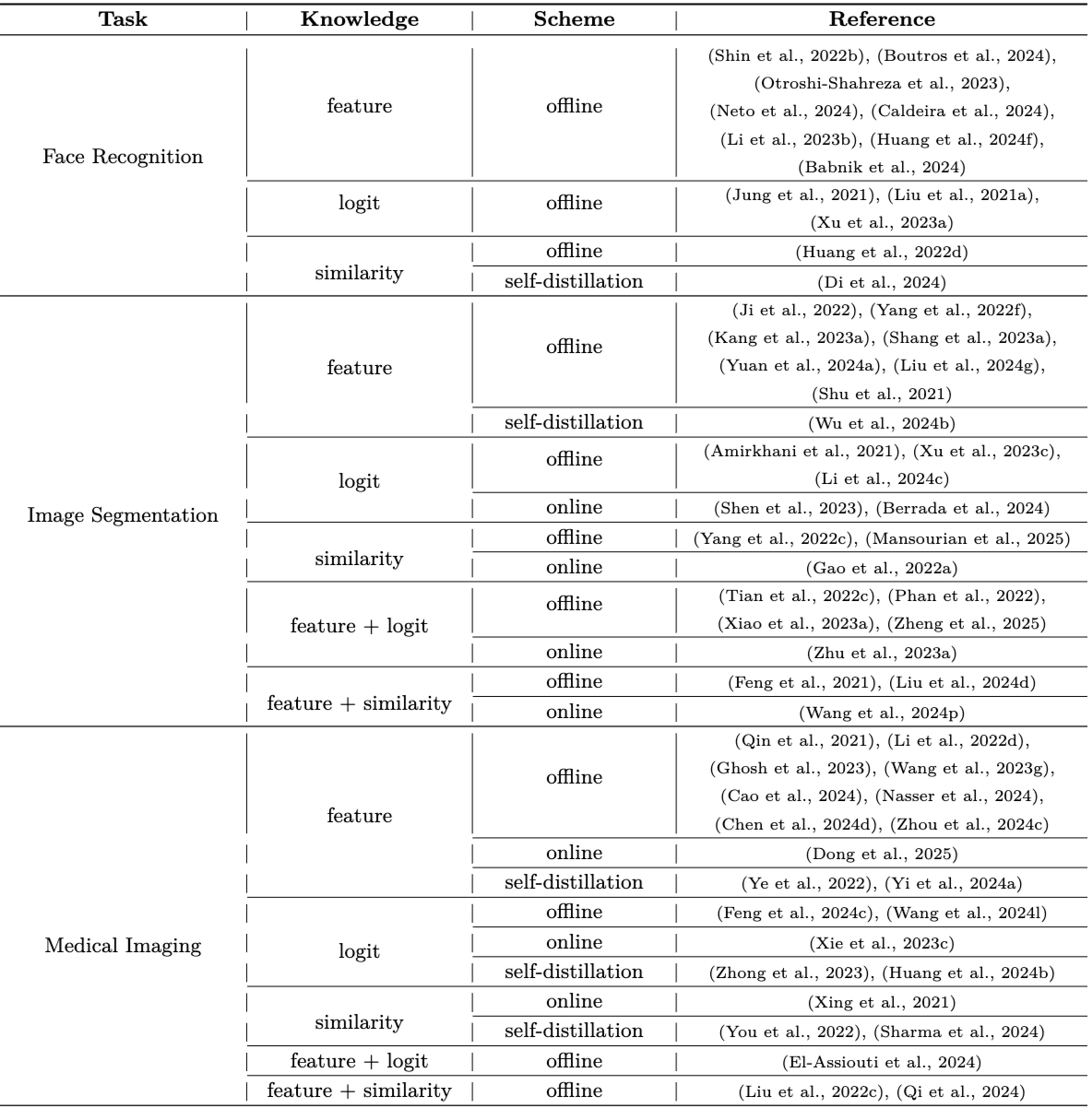
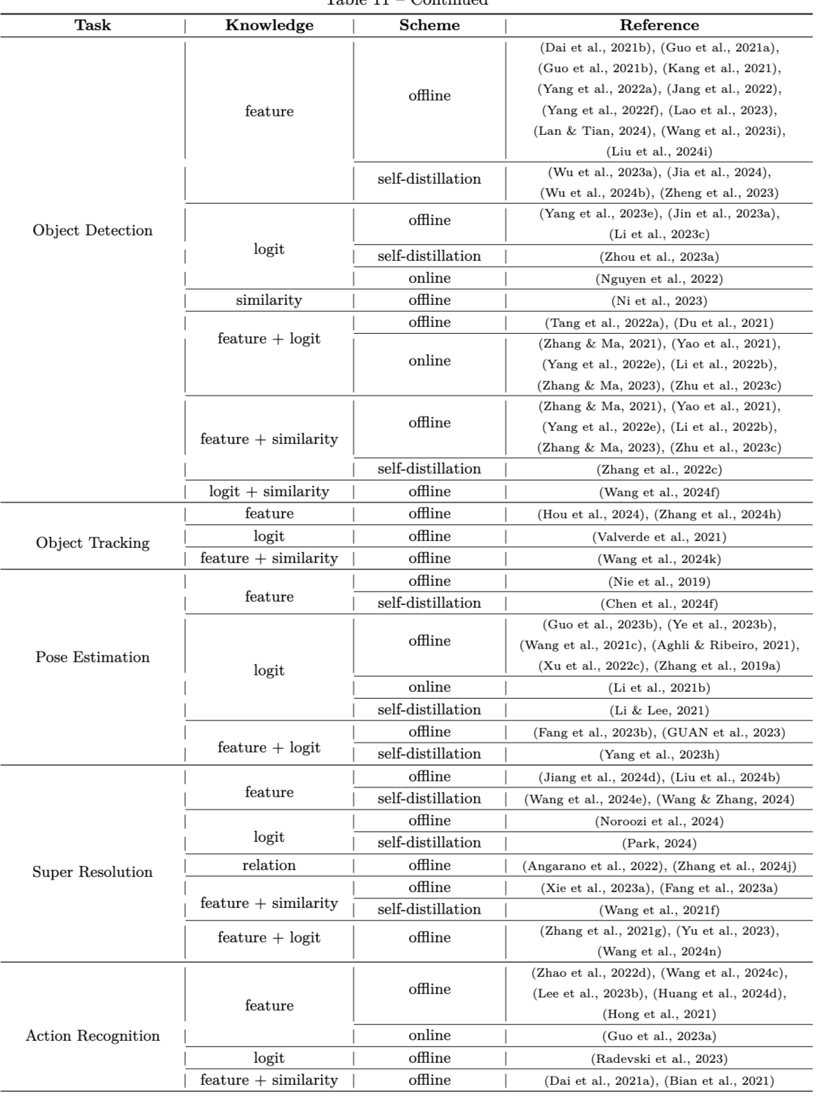
해당 논문의 Table 11

전통적인 CV task 전반에서 Source / Scheme taxonomy가 그대로 적용된다.

Large Teacher → Compact Student로 Teacher behavior를 유지하면서 computation과 memory를 줄이는 기본 목적이며, Table 11이 중심이다. Depth Estimation, Face Recognition, Image Segmentation, Medical Imaging, Object Detection, Object Tracking, Pose Estimation, Super Resolution, Action Recognition, Image Retrieval을 Knowledge Source + Distillation Scheme으로 정리한다.

Table 11에서 보이는 특징은

Source를 결합하는 경우가 많다 : Feature + Logit, Feature + Similarity, Similarity + Logit이 반복되며, 특히 segmentation, detection, super resolution에서 두드러진다.
- Image Segmentation : dense prediction이라 pixel-level feature + class/logit + spatial relation이 모두 유용해서 거의 모든 조합이 등장
- Object Detection : intermediate feature, logit, object relation 등을 조합하며 offline/online/self 모두 사용
Task에 따라 중요한 knowledge가 다르다
- Face Recognition : identity representation의 구조를 유지해야 해서 feature와 similarity
- Pose Estimation : logit이 heatmap 형태라 output-level knowledge도 충분히 informative하고 feature와 함께 사용
- Image Retrieval : class probability보다 embedding feature와 similarity structure가 핵심
Scheme도 다양하다 : segmentation, detection, medical, depth, pose, super resolution에서 self-distillation이, segmentation, detection, medical에서 online이 쓰이지만 여전히 offline이 가장 넓게 사용된다. (Discussion에서 본 내용과 일관)

Table 11은 어디에 어떤 KD가 사용되어 왔는가를 보여주는 표이지 Feature KD가 항상 Logit KD보다 낫다 같은 ranking table이 아니다.

Section 6.5의 역할
새로운 축을 제안하기보다 Source / Scheme taxonomy가 classification에만 국한되지 않고 실제 CV 전반에서 반복적으로 쓰인다는 coverage evidence인거 같다. 또한 taxonomy는 셋 중 하나를 고르는 메뉴가 아니라 Teacher knowledge를 분석하기 위한 기준이다. Discussion의 Table 17처럼 KD design은 context-dependent하고, task가 요구하는 representation에 맞게 knowledge source를 선택/결합하는 방향이 자연스럽다. Offline이 여전히 default인 이유도 전통 vision task에서는 strong pretrained Teacher를 준비하기 쉽기 때문이고, Self/Online은 Teacher pretraining cost를 피하거나 training 자체를 regularize하려는 상황에서 선택되는거 같다.

Applications 정리

KD의 역할이 얼마나 넓어졌는가
$\begin{aligned} \text{LLM} &: \text{Capability / Behavior Transfer} \\ \text{FM} &: \text{Downstream Knowledge Transfer / Capability Composition} \\ \text{SSL} &: \text{Representation Learning Mechanism} \\ \text{Diffusion} &: \text{Generation Process Compression} \end{aligned}$ 같은 Knowledge Distillation이라는 이름 아래에서도 실제로 전달되는 것이 완전히 달라졌다. 이것이 KD를 Large classifier → Small classifier로만 정의하기 어려운 가장 강한 근거인거 같다.

Section 7 : Performance Comparison

KD method의 clear & fair comparison은 거의 불가능하다.

Discussion에서 본 것처럼 KD 성능은 algorithm 하나로만 결정되지 않는다.

어떤 pretrained Teacher를 사용했는가 (Teacher weight)
epochs, batch size
Teacher-Student architecture
hardware resource
기타 training setting

그럼에도 비교가 가장 많이 이루어지는 task를 골라 표를 구성한다.

Classification : CIFAR-100, ImageNet
Semantic Segmentation : PascalVOC, Cityscapes
LLM : 여러 NLP / reasoning benchmark

1. Classification

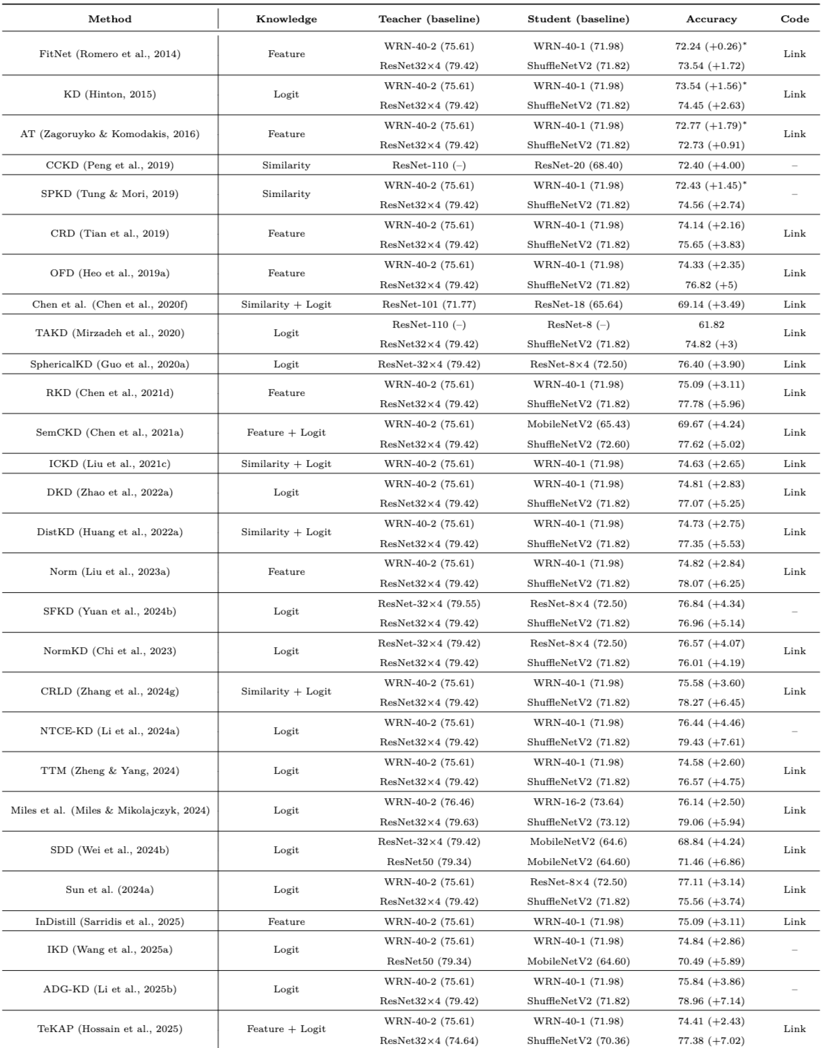
해당 논문의 Table 12

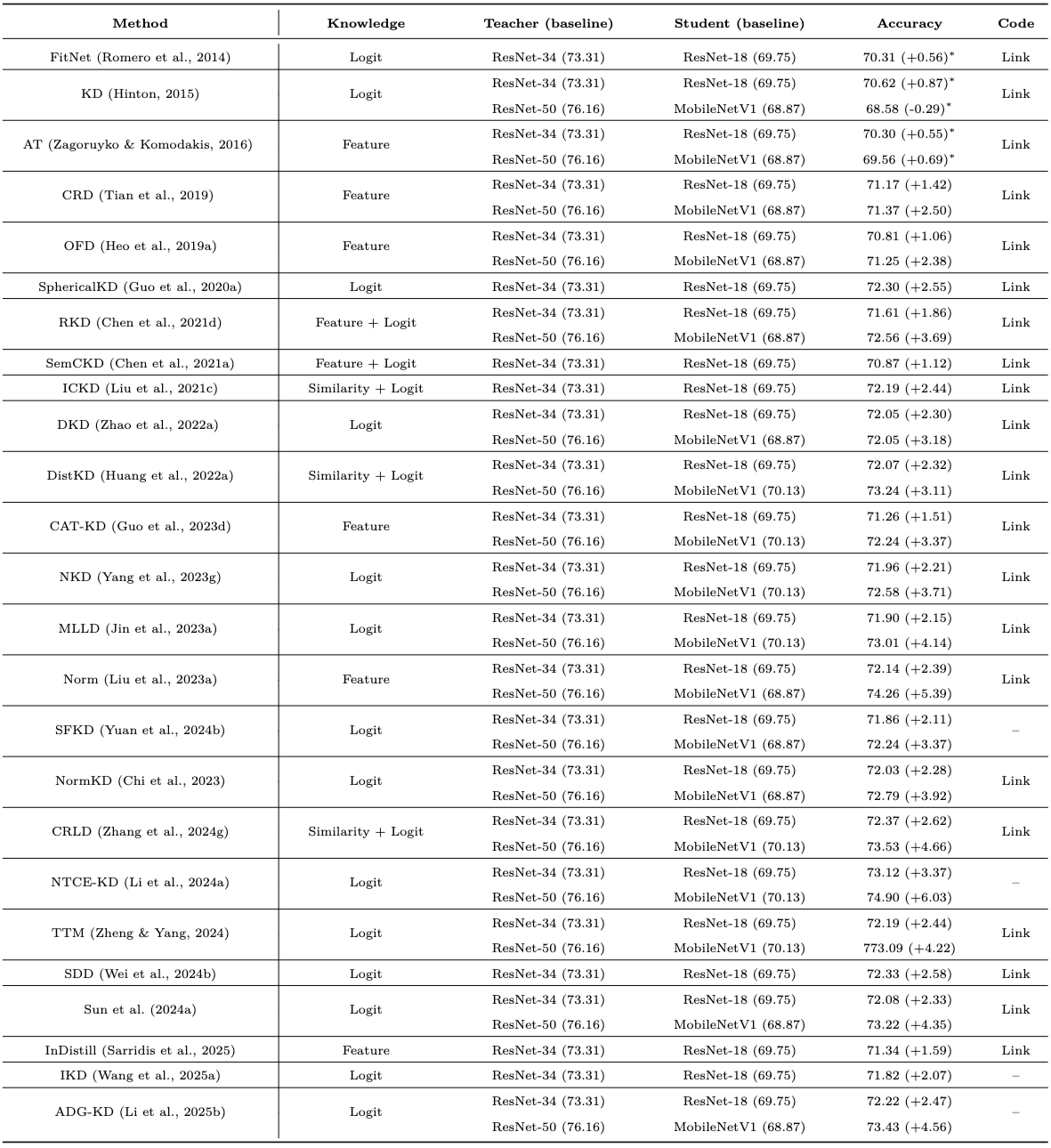
해당 논문의 Table 13

Knowledge Type + Teacher Baseline + Student Baseline + Post-KD Accuracy를 함께 보여주어 final accuracy뿐만 아니라 $\Delta = Acc(S_{\text{KD}}) - Acc(S_{\text{baseline}})$ 를 볼 수 있다. 또한 가능한 경우 두 setting을 모두 포함한다.

유사 architecture : WRN-40-2 → WRN-40-1
서로 다른 architecture : ResNet32×4 → ShuffleNetV2, ResNet-50 → MobileNetV1

CIFAR-100 (Table 12) 는 FitNet, Vanilla KD, AT, SPKD 같은 초기 method부터 CRD, OFD, RKD, SemCKD, DKD, DistKD, Norm, CRLD, NTCE-KD, ADG-KD 등 2025년 method까지 포함하며, 후기 method에서 더 큰 Student improvement가 보고된다. 하지만 강한 결과가 Feature에서도, Logit에서도, Similarity + Logit에서도 나타나서 표만으로 Feature가 항상 최고라고 결론 내릴 수 없다.

ImageNet (Table 13) 도 비슷하게 초기 method는 작은 improvement, 이후 method는 더 큰 gain을 보인다. 특히 heterogeneous setting에서도 여러 method가 Student baseline을 크게 개선하여 architecture가 다른 Teacher-Student에서도 KD가 유효하다는 evidence가 된다. 다만 method별 sensitivity가 커서 Discussion에서 여전히 challenge로 남는다.

2. Semantic Segmentation

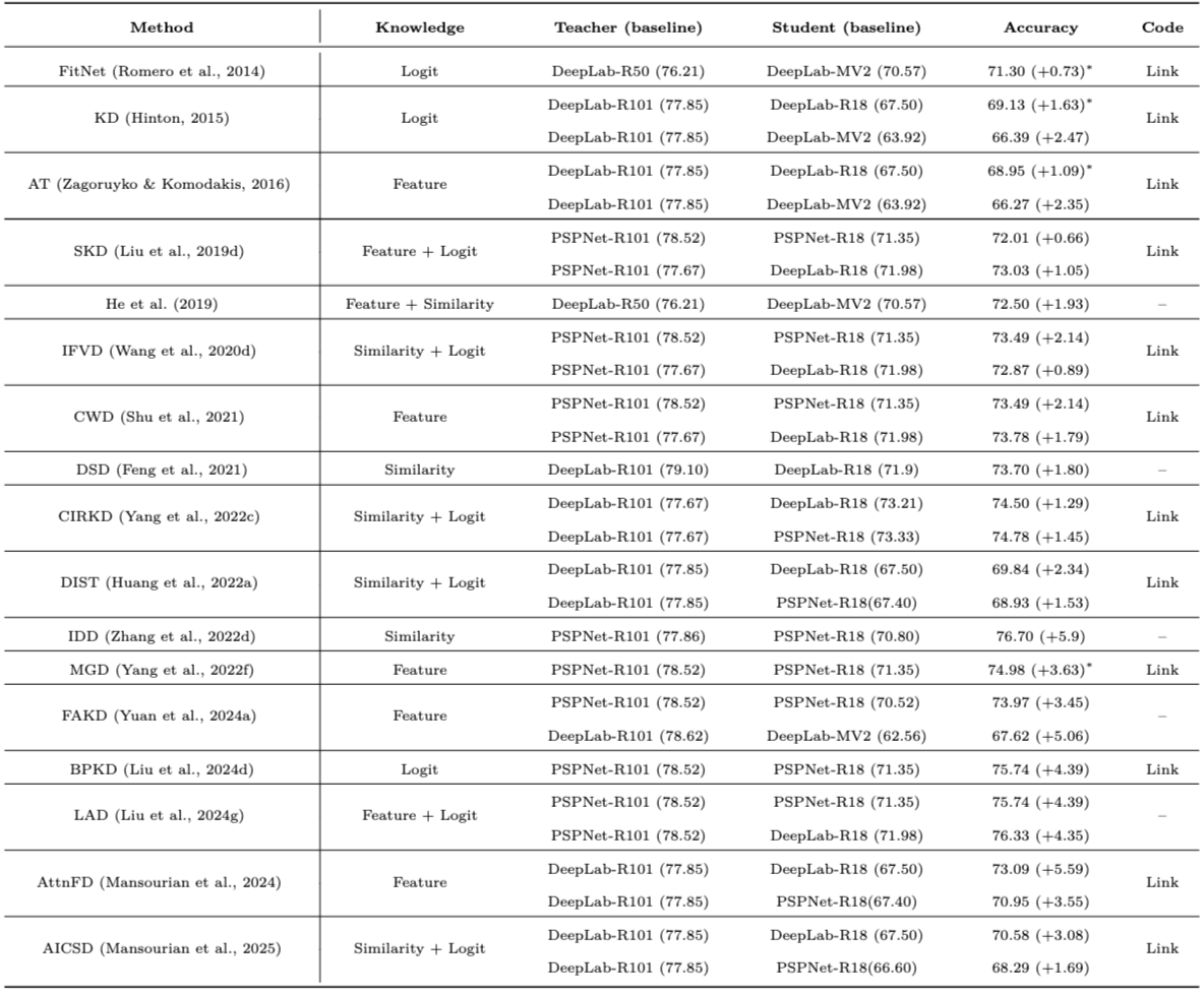
해당 논문의 Table 14

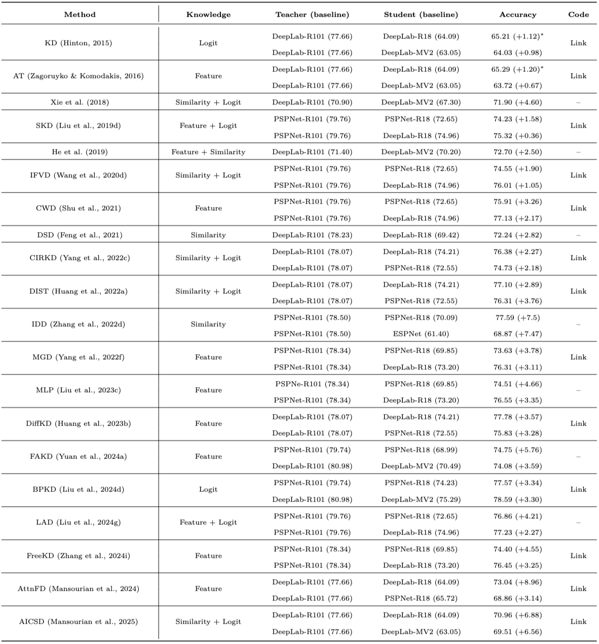
해당 논문의 Table 15

PascalVOC와 Cityscapes에서 Vanilla KD, AT부터 CWD, CIRKD, DIST, MGD, FAKD, BPKD, LAD, AttnFD, AICSD까지 비교한다. dense prediction에서는 Feature와 Similarity를 쓰는 method의 비중이 classification보다 두드러진다. pixel / region / channel / class relation 같은 intermediate structural knowledge가 segmentation에서 유용하기 때문이다. DeepLab-R101 → DeepLab-R18 같은 유사 family뿐만 아니라 PSPNet-R101 → DeepLab-R18 같은 다른 architecture setting도 포함하며, 저자들은 이 정보가 dataset size와 architectural difference에 대한 robustness를 판단하는 데 도움이 된다고 설명한다.

Table 12 ~ 15의 * 표기
*가 붙은 결과는 원 논문에 해당 setting 결과가 없어서 survey 저자들이 직접 구현한 결과이다. 즉 같은 표 안에 original reported result와 survey reproduction이 섞여 있어서, 작은 accuracy 차이로 $A > B$라고 해석하는 것은 더 위험하다. 정확한 leaderboard가 아니라 landscape comparison에 가깝다.

3. LLM

LLM은 vision보다 비교가 더 어렵다. Teacher, Student, benchmark, model size, distillation type이 연구마다 크게 다르기 때문이다. 그래서 Table 16은 White-box와 Black-box를 나누고 Compression Rate + Benchmark Performance를 함께 보여준다.

White-box : DistilBERT, TinyBERT, PKD, MobileBERT, MiniLM, TED, MiniLLM, GKD 등에서 높은 compression rate와 비교적 작은 performance degradation을 동시에 얻는다.
Black-box : ICL / IF / CoT로 나누며 Teacher가 GPT-3.5, GPT-175B, PaLM-540B, Gemini 등이라 Student와의 parameter gap이 훨씬 크다. * row는 Student 전/후 비교이므로 모든 percentage를 같은 의미의 $\frac{\text{Student}}{\text{Teacher}}$로 보면 안 된다.

저자들은 어떤 method가 다른 method보다 우수하다고 직접 주장하지 않는다고 명시한다. 대신 이 표들로

다양한 dataset에서 KD가 Student를 얼마나 개선하는지
동일 / 이질 architecture에서 어떻게 동작하는지
각 method가 어떤 knowledge source를 쓰는지
compression 후 Teacher performance를 어느 정도 유지하는지

를 참고할 수 있게 한다.

그래도 Future Direction에서 Feature based가 최근 Student 성능 향상에서 강한 결과를 보인다는 qualitative 판단은 한다. 표에서도 Feature Transformation, Similarity + Logit, Decoupled Logit, Adaptive/Attention Feature 같은 richer strategy가 Vanilla KD보다 큰 improvement를 보고하는 경우가 많다. 하지만 controlled experiment가 아니므로 정확한 causality나 ranking은 주장할 수 없다.

Performance Section에서 말할 수 있는 수준
이 Section은 현재 SOTA KD는 무엇인가?에 답하는 곳이 아니라 KD 성능은 method 이름 하나만으로 설명할 수 없다는 것을 보여주는 곳인거 같다. 어떤 paper의 +7%가 다른 paper의 +4%보다 method가 우수하다는 뜻은 아니다. 안전하게 말할 수 있는 것은
1 2 Vanilla Output Mimicking → 더 정교한 Feature / Relation / Logit Manipulation 이 꾸준히 연구되었고 단순 KD보다 큰 Student improvement를 보고하는 연구가 많아졌다
정도이다. LLM에서도 GLUE, GSM8K, MATH처럼 측정하는 capability 자체가 다르므로 compression rate가 크다 ≠ Teacher capability가 잘 보존됐다이다.

Section 2 ~ 7을 하나로 연결하면
Knowledge Source의 확장 : Logit → Feature → Relation / Structure
Teacher 정의의 확장 : External Large Teacher → Peer / Self → Multiple Teachers → Other Modality / FM
Transfer Mechanism의 정교화 : Direct Matching → Attention / Adversarial / Graph → Adaptive / Contrastive
KD 역할의 확장 $\text{Compression} \rightarrow \text{Supervision Transfer} \rightarrow \text{Representation Learning} \rightarrow \text{Capability Transfer} \rightarrow \text{Generation Process Acceleration}$
그리고 Section 7은 이 발전을 단순 accuracy leaderboard로 설명할 수 없다는 것을 알려준다.

어떤 loss가 가장 높은 숫자를 내는가 → Teacher의 어떤 knowledge를 어떤 Student에게 어떤 조건에서 전달할 것인가

AI-ML-DL, etc.

Knowledge-Distillation

This post is licensed under CC BY 4.0 by the author.